AWS Big Data Blog
Create, train, and deploy machine learning models in Amazon Redshift using SQL with Amazon Redshift ML
December 2022: Post was reviewed and updated to announce support of Prediction Probabilities for Classification problems using Amazon Redshift ML.
Amazon Redshift is a fast, petabyte-scale cloud data warehouse data warehouse delivering the best price–performance. Tens of thousands of customers use Amazon Redshift to process exabytes of data every day to power their analytics workloads. Data analysts and database developers want to use this data to train machine learning (ML) models, which can then be used to generate insights on new data for use cases such as forecasting revenue, predicting customer churn, and detecting anomalies.
Amazon Redshift ML makes it easy for SQL users to create, train, and deploy ML models using familiar SQL commands. Redshift ML allows you to use your data in Amazon Redshift with Amazon SageMaker, a fully managed ML service, without requiring you to become an expert in ML.
This post shows you how to use familiar SQL statements to create and train ML models from data in Amazon Redshift and use these models to make in-database predictions on new data for use cases such as churn prediction and fraud risk scoring.
ML use cases relevant to data warehousing
You may use different ML approaches according to what’s relevant for your business, such as supervised, unsupervised, and reinforcement learning. With this release, Redshift ML supports supervised learning, which is most commonly used in enterprises for advanced analytics. As evident in the following diagram, supervised learning is preferred when you have a training dataset and an understanding of how specific input data predicts various business outcomes. The inputs used for the ML model are often referred to as features, and the outcomes or results are called targets or labels. Your training dataset is a table or a query whose attributes or columns comprise features, and targets are extracted from your data warehouse. The following diagram illustrates this architecture.
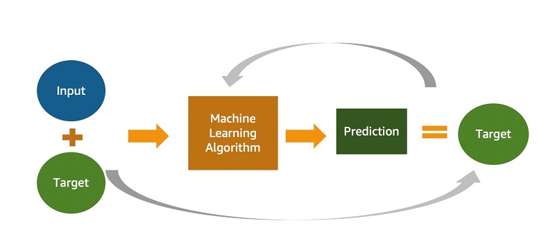
You can use supervised training for advanced analytics use cases ranging from forecasting and personalization to customer churn prediction. Let’s consider a customer churn prediction use case. The columns that describe customer information and usage are features, and the customer status (active vs. inactive) is the target or label.
The following table shows different types of use cases and algorithms used.
| Use Case | Algorithm / Problem Type |
| Customer churn prediction | Classification |
| Predict if a sales lead will close | Classification |
| Fraud detection | Classification |
| Price and revenue prediction | Linear regression |
| Customer lifetime value prediction | Linear regression |
| Detect if a customer is going to default a loan | Logistic regression |
Current ways to use ML in your data warehouse
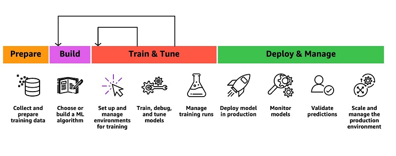
You may rely on ML experts to build and train models on your behalf or invest a lot of time into learning new tools and technology to do so yourself. For example, you might need to identify the appropriate ML algorithms in SageMaker or use Amazon SageMaker Autopilot for your use case, then export the data from your data warehouse and prepare the training data to work with these model types.
Data analysts and database developers are familiar with SQL. Unfortunately, you often have to learn a new programming language (such as Python or R) to build, train, and deploy ML models in SageMaker. When the model is deployed and you want to use it with new data for making predictions (also known as inference), you need to repeatedly move the data back and forth between Amazon Redshift and SageMaker through a series of manual and complicated steps:
- Export training data to Amazon Simple Storage Service (Amazon S3).
- Train the model in SageMaker.
- Export prediction input data to Amazon S3.
- Use the prediction in SageMaker.
- Import predicted columns back into the database.
The following diagram illustrates this workflow.
This iterative process is time-consuming and prone to errors, and automating the data movement can take weeks or months of custom coding that then needs to be maintained. Redshift ML enables you to use ML with your data in Amazon Redshift without this complexity.
Introducing Amazon Redshift ML
To create an ML model, as a data analyst, you can use a simple SQL query to specify the data in Amazon Redshift you want to use as the data inputs to train your model and the output you want to predict. For example, to create a model that predicts customer churn, you can query columns in one or more tables in Amazon Redshift that include the customer profile information and historical account activity as the inputs, and the column showing whether the customer is active or inactive as the output you want to predict.
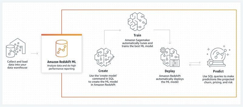
When you run the SQL command to create the model, Redshift ML securely exports the specified data from Amazon Redshift to Amazon S3 and calls Autopilot to automatically prepare the data, select the appropriate pre-built algorithm, and apply the algorithm for model training. Redshift ML handles all the interactions between Amazon Redshift, Amazon S3, and SageMaker, abstracting the steps involved in training and compilation. After the model is trained, Redshift ML makes it available as a SQL function in your Amazon Redshift data warehouse by compiling it via Amazon SageMaker Neo. The following diagram illustrates this solution.
Benefits of Amazon Redshift ML
Redshift ML provides the following benefits:
- Allows you to create and train ML models with simple SQL commands without having to learn external tools
- Provides you with flexibility to use automatic algorithm selection
- Automatically preprocesses data and creates, trains, and deploys models
- Enables advanced users to specify problem type
- Enables ML experts such as data scientists to select algorithms such as XGBoost or MLP and specify hyperparameters and preprocessors
- Enables you to generate predictions using SQL without having to ship data outside your data warehouse
- Allows you to pay only for training; prediction is included with the costs of your cluster (typically, ML predictions drive cost in production)
In this post, we look at a simple example that you can use to get started with Redshift ML.
To train data for a model that predicts customer churn, Autopilot preprocesses the training data, finds the algorithm that provides the best accuracy, and applies it to the training data to build a performant model.
We provide step-by-step guidance to create a cluster, create sample schema, load data, create your first ML model in Amazon Redshift, and invoke the prediction function from your queries.
Prerequisites for enabling Amazon Redshift ML
As an Amazon Redshift administrator, the following steps are required to create your Amazon Redshift cluster for using Redshift ML:
- On the Amazon S3 console, create an S3 bucket that Redshift ML uses for uploading the training data that SageMaker uses to train the model.
For this post, we name the bucket redshiftml-<your_account_id>. Make sure that you create your S3 bucket in the same AWS Region where you create your Amazon Redshift cluster.
- Create an AWS Identity and Access Management (IAM role) named
RedshiftMLwith the policy that we provide in this section.
Although it’s easy to get started with AmazonS3FullAccess and AmazonSageMakerFullAccess, we recommend using the minimal policy that we provided (if you already have an existing IAM role, just add these to that role). Take a look at the Amazon Redshift ML guide if you need to use KMS or enhanced VPC routing.
To use or modify this policy, replace <your-account-id> with your AWS account number. The policy assumes that you have created the IAM role RedshiftML and the S3 bucket redshiftml-<your_account_id>. The S3 bucket redshift-downloads is from where we load the sample data used in this post.
For instructions, see Creating IAM roles.
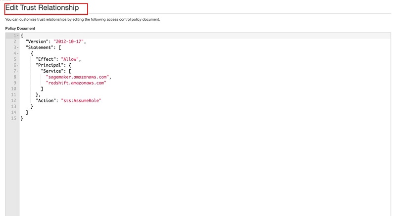
- On the role details page, on the Trust relationships tab, choose Edit trust relationship.

- Enter the following trust relationship definition to trust SageMaker:
- On the Amazon Redshift console, create a new Amazon Redshift cluster.
- Attach the IAM role that you created earlier (
RedshiftML). - Create the cluster with the current track.

When your cluster creation is complete and the cluster is up and running, you can create accounts for data analysts on an Amazon Redshift cluster. For this post, we create a user named demouser.
- Use the Amazon Redshift Query Editor or your preferred SQL client to connect to Amazon Redshift as an administrator and run the following command:
Alternately we have provided a notebook you may use to execute all the sql commands that can be downloaded here. You will find instructions in this blog on how to import and use notebooks. - Grant CREATE MODEL privileges to your users. The following code grants privileges to the
demouseruser for creating a model:
Loading sample data
We use a customer churn model in this post. As an admin or database developer, you have to create the schema and load data into Amazon Redshift. This dataset is attributed to the University of California Irvine Repository of Machine Learning Datasets (Jafari-Marandi, R., Denton, J., Idris, A., Smith, B. K., & Keramati, A. (2020). Optimum Profit-Driven Churn Decision Making: Innovative Artificial Neural Networks in Telecom Industry. Neural Computing and Applications). We have modified this data for use with Redshift ML.
- Create a schema named
demo_mlthat stores the example table and the ML model that we create:
In the next steps, we create the sample table and load data into the table that we use to train the ML model.
- Create the table in the
demo_mlschema: - Load the sample data by using the following command. Replace your IAM role and account ID appropriate for your environment.
- The
demouseruser should also have the usual SELECT access to the tables with the data used for training:
- You need to also grant CREATE and USAGE on the schema to allow users to create models and query using the ML inference functions on the demo_ml schema:
Now the analyst (demouser) can train a model.
Create and train your first ML model
Use your preferred SQL client to connect to your Amazon Redshift cluster as the demouser user that your admin created. Run the following command to create your model named customer_churn_model:
The SELECT query in the FROM clause specifies the training data. The TARGET clause specifies which column is the label that the CREATE MODEL builds a model to predict. The other columns in the training query are the features (input) used for the prediction. In this example, the training data provides features regarding state, area code, average daily spend, and average daily cases for the customers that have been active earlier than January 1, 2020. The target column churn indicates whether the customer still has an active membership or has suspended their membership. For more information about CREATE MODEL syntax, see the Amazon Redshift Database Developer Guide.
With recent enhancements, Redshift ML now supports Prediction Probabilities for binary and multi-class classification models. For classification problems in machine learning, for a given record, each label can be associated with a probability that indicates how likely this record belongs to the label. Having prediction probabilities along with the label, customers could use the classification results with confidence based on a certain threshold value of prediction probability returned by the model.
Prediction probabilities are calculated by default for binary and multi-class classification models; there is no extra parameter needs to be passed while creating a model and an additional function is created while creating a model without impacting performance of the ML model.
Check the status of your ML model
You can check the status of your models by running the SHOW MODEL command from your SQL prompt. Enter the SHOW MODEL ALL command to see all the models that you have access to:
The following table summarizes our output.
| SchemaName | ModelName |
demo_ml |
customer_churn_model |
Enter the SHOW MODEL command with your model name to see the status for a specific model:
The following output provides the status of your model:
As highlighted in bold above, predication probabilities enhancements have added another function as a suffix (_prob) to model function which could be used to get prediction probabilities
Evaluate your model performance
You can see the F1 value for the example model customer_churn_model in the output of the SHOW MODEL command. The F1 amount signifies the statistical measure of the precision and recall of all the classes in the model. The value ranges between 0–1; the higher the score, the better the accuracy of the model.
You can use the following example SQL query as an illustration to see which predictions are incorrect based on the ground truth:
You can change the above SQL query to get prediction probabilities of each of the label returned.
Here is sample output of above query which shows customer churn prediction along with values of prediction probabilities mapped to each of the possible label values.
We can also observe that Redshift ML is able to identify the right combination of features to come up with a usable prediction model with Model Explainability. Model explainability helps explain how these models make predictions using a feature attribution approach which in turn helps improve your machine learning (ML) models. We can check impact of each attribute and its contribution and weightage in the model selection using the following command:
The following output is from the above command, where each attribute weightage is representative of its role in the model decision-making.
Invoke your ML model for inference
You can use your SQL function to apply the ML model to your data in queries, reports, and dashboards. For example, you can run the predict_customer_churn SQL function on new customer data in Amazon Redshift regularly to predict customers at risk of churning and feed this information to sales and marketing teams so they can take preemptive actions, such as sending these customers an offer designed to retain them.
For example, you can run the following query to predict which customers in area code 408 might churn:
The following output shows the account ID and whether the account is predicted to remain active.
| accountId | predictedActive |
408393-7984 |
False. |
408357-3817 |
True. |
408418-6412 |
True. |
408395-2854 |
True. |
408372-9976 |
False. |
408353-3061 |
True. |
Additionally, you can change the above query to include prediction probabilities of label output for the above scenario and decide if you still like to use the prediction by the model.
Provide privileges to invoke the prediction function
As the model owner, you can grant EXECUTE on the prediction function to business analysts to use the model. The following code grants the EXECUTE privilege to marketing_analyst_grp:
Cost control
Redshift ML uses your existing cluster resources for prediction so you can avoid additional Amazon Redshift charges. There is no additional Amazon Redshift charge for creating or using a model, and prediction happens locally in your Amazon Redshift cluster, so you don’t have to pay extra unless you need to resize your cluster.
The CREATE MODEL request uses SageMaker for model training and Amazon S3 for storage, and incurs additional expense. The cost depends on the number of cells in your training data; the number of cells is the product of the number of records (in the training query or table) times the number of columns. For example, if the SELECT query of CREATE MODEL produces 10,000 records for training and each record has five columns, the number of cells in the training data is 50,000. You can control the training cost by setting the MAX_CELLS. If you don’t, the default value of MAX_CELLS is 1 million.
If the training data produced by the SELECT query of the CREATE MODEL exceeds the MAX_CELLS limit you provided (or the default 1 million, in case you didn’t provide one) the CREATE MODEL randomly chooses approximately MAX_CELLS divided by number of columns records from the training dataset and trains using these randomly chosen tuples. The random choice ensures that the reduced training dataset doesn’t have any bias. Therefore, by setting the MAX_CELLS, you can keep your cost within your limits. See the following code:
For more information about costs associated with various cell numbers and free trial details, see Amazon Redshift pricing.
An alternate method of cost control is the MAX_RUNTIME parameter, also specified as a CREATE MODEL setting. If the training job in SageMaker exceeds the specified MAX_RUNTIME seconds, the CREATE MODEL ends the job.
The prediction functions run within your Amazon Redshift cluster, and you don’t incur additional expense there.
Customer feedback
“We use predictive analytics and machine learning to improve operational and clinical efficiencies and effectiveness. With Redshift ML, we enabled our data and outcomes analysts to classify new drugs to market into appropriate therapeutic conditions by creating and utilizing ML models with minimal effort. The efficiency gained through leveraging Redshift ML to support this process improved our productivity and optimized our resources.”
– Karim Prasla, Vice President of Clinical Outcomes Analytics and Reporting, Magellan Rx Management
“Jobcase has several models in production using Amazon Redshift Machine Learning. Each model performs billions of predictions in minutes directly on our Redshift data warehouse with no data pipelines required. With Redshift ML, we have evolved to model architectures that generate a 5-10% improvement in revenue and member engagement rates across several different email template
types, with no increase in inference costs.”
– Mike Griffin, EVP Optimization & Analytics, Jobcase
Please refer to blog posts for Magellan Rx and Jobcase to learn more.
Conclusion
In this post, we briefly discussed ML use cases relevant for data warehousing. We introduced Redshift ML and outlined how it enables SQL users to create, train, deploy, and use ML with simple SQL commands without learning external tools. We also provided an example of how to get started with Redshift ML.
Redshift ML also enables ML experts such as data scientists to quickly create ML models to simplify their pipeline and eliminate the need to export data from Amazon Redshift. In the following posts, we discuss how you can use Redshift ML to import your pre-trained Autopilot, XGBoost, or MLP models into your Amazon Redshift cluster for local inference or use custom ML models deployed in remote SageMaker endpoints for remote inference. With recent Redshift ML enhancement of prediction probabilities now customer could use prediction by binary and multi-class classification prediction with the confidence level of the label predicted without any additional costs.
About the Authors
 Debu Panda, a principal product manager at AWS, is an industry leader in analytics, application platform, and database technologies and has more than 20 years of experience in the IT world.
 Yannis Papakonstantinou is a senior principal scientist at AWS and professor (on leave) of University of California at San Diego whose research on querying nested and semi-structured data, data integration, and the use and maintenance of materialized views has received over 16,500 citations.
 Murali Balakrishnan Narayanaswamy is a principal machine learning scientist at AWS and received a PhD from Carnegie Mellon University on the intersection of AI, optimization, learning and inference to combat uncertainty in real-world applications.
 Sriram Krishnamurthy is a senior software development manager for the Amazon Redshift query processing team and has been working on semi-structured data processing and SQL compilation and execution for over 15 years.
 Sudipta Sengupta is a senior principal technologist at AWS who leads new initiatives in AI/ML, databases, and analytics and holds a Ph.D. in electrical engineering and computer science from Massachusetts Institute of Technology.
 Stefano Stefani is a VP and distinguished engineer at AWS and has served as chief technologist for Amazon DynamoDB, Amazon Redshift, Amazon Aurora, Amazon SageMaker, and other services.
 Rohit Bansal is an Analytics Specialist Solutions Architect at AWS. He specializes in Amazon Redshift and works with customers to build next-generation analytics solutions using other AWS Analytics services.
 Phil Bates is a Senior Analytics Specialist Solutions Architect at AWS with over 25 years of data warehouse experience.