AWS Machine Learning Blog
Estimating the Location of Images Using Apache MXNet and Multimedia Commons Dataset on AWS EC2
This is a guest post by Jaeyoung Choi of the International Computer Science Institute and Kevin Li of the University of California, Berkeley. This project demonstrates how academic researchers can leverage our AWS Cloud Credits for Research Program to support their scientific breakthroughs.
Modern mobile devices can automatically assign geo-coordinates to images when you take pictures of them. However, most images on the web still lack this location metadata. Image geo-location is the process of estimating the location of an image and applying a location label. Depending on the size of your dataset and how you pose the problem, the assigned location label can range from the name of a building or landmark to an actual geo-coordinate (latitude, longitude).
In this post, we show how to use a pre-trained model created with Apache MXNet to geographically categorize images. We use images from a dataset that contains millions of Flickr images taken around the world. We also show how to map the result to visualize it.
Our approach
The approaches to image geo-location can be divided into two categories: image-retrieval-based search approaches and classification-based approaches. (This blog post compares two state-of-the-art approaches in each category.)
Recent work by Weyand et al. posed image geo-location as a classification problem. In this approach, the authors subdivided the surface of the earth into thousands of geographic cells and trained a deep neural network with geo-tagged images. For a less technical description of their experiment, see this article.
Because the authors did not release their training data or their trained model, PlaNet, to the public, we decided to train our own image geo-locator. Our setup for training the model is inspired by the approach described in Weyand et al., but we changed several settings.
We trained our model, LocationNet, using MXNet on a single p2.16xlarge instance with geo-tagged images from the AWS Multimedia Commons dataset.
We split training, validation, and test images so that images uploaded by the same person do not appear in multiple sets. We used Google’s S2 Geometry Library to create classes with the training data. The model converged after 12 epochs, which took about 9 days with the p2.16xlarge instance. A full tutorial with a Jupyter notebook is available on GitHub.
The following table compares the setups used to train and test LocationNet and PlaNet.
| LocationNet | PlaNet | |
| Dataset source | Multimedia Commons | Images crawled from the web |
| Training set | 33.9 million | 91 million |
| Validation | 1.8 million | 34 million |
| S2 Cell Partitioning | t1=5000, t2=500 → 15,527 cells |
t1=10,000, t2=50 → 26,263 cells |
| Model | ResNet-101 | GoogleNet |
| Optimization | SGD with Momentum and LR Schedule | Adagrad |
| Training time | 9 days on 16 NVIDIA K80 GPUs (p2.16xlarge EC2 instance), 12 epochs |
2.5 months on 200 CPU cores |
| Framework | MXNet | DistBelief |
| Test set | Placing Task 2016 Test Set (1.5 million Flickr images) | 2.3 M geo-tagged Flickr images |
At inference time, LocationNet outputs a probability distribution over the geographic cells. The center-of-mass geo-coordinate of the images in the cell with the highest likelihood is assigned as the geo-coordinate of the query image.
LocationNet is shared publicly in the MXNet Model Zoo.
Downloading LocationNet
Now download LocationNet, the pretrained model. LocationNet has been trained on the subset of geo-tagged images in the AWS Multimedia Commons dataset. The Multimedia Commons dataset contains more than 39 million images and 15 thousand geographic cells (classes).
LocationNet has two parts, a JSON file containing the model definition and a binary file containing the parameters. We load necessary packages and download the files from S3.
Then, load the downloaded model. If you don’t have a GPU available, replace mx.gpu() with mx.cpu():
The grids.txt file contains the geographic cells used for training the model.
The i-th line is the i-th class, and the columns are: S2 Cell Token, Latitude, and Longitude. We load the labels to a list named grids.
Before feeding the image to the deep learning network, the model preprocesses the image by cropping it and subtracting the mean:
Evaluating and comparing models
For evaluation, we use two datasets: the IM2GPS dataset and a test dataset of Flickr images that is used in MediaEval Placing 2016 Benchmark.
Results for the IM2GPS test set
The following values indicate the percentage of images in the IM2GPS test set that were correctly located within each distance from the actual location.
| Method | 1km | 25km | 200km | 750km | 2500km |
| PlaNet | 8.4% | 24.5% | 37.6% | 53.6% | 71.3% |
| LocationNet | 16.8% | 39.2% | 48.9% | 67.9% | 82.2% |
Results for Flickr images
These results are not directly comparable because the test set images used in PlaNet have not been publicly released. The values indicate the percentage of images in the test set that were correctly located within each distance from the actual location.
| Method | 1km | 25km | 200km | 750km | 2500km |
| PlaNet | 3.6% | 10.1% | 16.0% | 28.4% | 48.0% |
| LocationNet | 6.2% | 13.5% | 20.8% | 35.6% | 55.2% |
By visually inspecting the geo-located images, we can see that the model does well with landmark locations, but it is also capable of correctly geo-locating non-landmark scenes.
Estimating the geo-location of an image using a URL
Now let’s try to geo-locate an image on the web using a URL .
Let’s see how our model does with an image of Tokyo Tower. The following code downloads the image from URL and outputs the model’s location prediction.

![]()
The result lists the top-5 result with the confidence score (prob) and the geo-coordinate:
It is hard to tell the quality of the geo-location output with just the raw latitude and longitude values. Let’s map the output to visualize the results.
Visualizing results using Google Maps on the Jupyter notebook
To visualize the results of the prediction, we use Google Maps in the Jupyter notebook. This allows you to see if the prediction makes sense. We use a plugin called gmaps, which allows the use of Google Maps in the Jupyter Notebook. To install gmaps, follow the installation instructions on the gmaps GitHub page.
Visualizing the result with gmaps takes only a few lines of code. In your notebook, type the following:
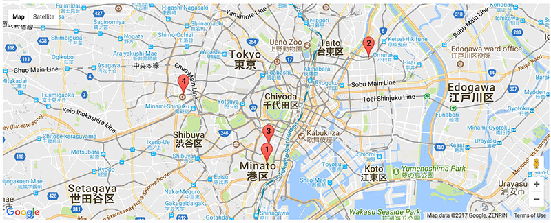
The top-1 geo-location estimation result is, indeed, right on the spot where Tokyo Tower is.
Now, try to geo-locate images of your choice!
Acknowledgements
Training LocationNet on AWS has been graciously supported by AWS Programs for Research and Education. We also thank the AWS Public Dataset program for hosting the Multimedia Commons dataset for public use. Our work is also partially supported by a collaborative LDRD led by Lawrence Livermore National Laboratory (U.S. Dept. of Energy contract DE-AC52-07NA27344).
Additional Reading
Learn more about AWS Cloud Credits for Research! Read about Ottertune and how to tune your DBMS automatically with Machine Learning.