Best Practices for Amazon Redshift Spectrum

November 2022: This post was reviewed and updated for accuracy.

Amazon Redshift Spectrum enables you to run Amazon Redshift SQL queries on data that is stored in Amazon Simple Storage Service (Amazon S3). With Amazon Redshift Spectrum, you can extend the analytic power of Amazon Redshift beyond the data that is stored natively in Amazon Redshift.

Amazon Redshift Spectrum offers several capabilities that widen your possible implementation strategies. For example, it expands the data size accessible to Amazon Redshift and enables you to separate compute from storage to enhance processing for mixed-workload use cases.

Amazon Redshift Spectrum also increases the interoperability of your data, because you can access the same S3 object from multiple compute platforms beyond Amazon Redshift. Such platforms include Amazon Athena, Amazon EMR with Apache Spark, Amazon EMR with Apache Hive, Presto, and any other compute platform that can access Amazon S3. You can query vast amounts of data in your Amazon S3 data lake without having to go through a tedious and time-consuming extract, transfer, and load (ETL) process. You can also join external Amazon S3 tables with tables that reside locally on Amazon Redshift. Amazon Redshift Spectrum applies sophisticated query optimization and scales processing across thousands of nodes to deliver fast performance.

In this post, we collect important best practices for Amazon Redshift Spectrum and group them into several different functional groups. We base these guidelines on many interactions and considerable direct project work with Amazon Redshift customers.

Before you get started, there are a few setup steps. For more information about prerequisites to get started in Amazon Redshift Spectrum, see Getting started with Amazon Redshift Spectrum. Please also refer to Define error handling for Amazon Redshift Spectrum data blog to understand how to handle data errors in Redshift Spectrum.

Set up the test environment

To perform tests to validate the best practices we outline in this post, you can use any dataset. Amazon Redshift Spectrum supports many common data formats: text, Parquet, ORC, JSON, Avro, and more. You can query data in its original format or convert data to a more efficient one based on data access pattern, storage requirement, and so on. For example, if you often access a subset of columns, a columnar format such as Parquet and ORC can greatly reduce I/O by reading only the needed columns. How to convert from one file format to another is beyond the scope of this post. For more information on how this can be done, see the following resources:

The Amazon Redshift data lake export feature
The aws-blog-spark-parquet-conversion AWS Samples GitHub repo
Converting to columnar formats (using Amazon EMR with Apache Hive for conversion)
Visualize AWS CloudTrail Logs Using AWS Glue and Amazon QuickSight

Create an external schema

You can create an external schema named s3_external_schema as follows:

create external schema s3_external_schema 
from data catalog 
database 'spectrumdb' 
iam_role 'arn:aws:iam::<AWS_ACCOUNT_ID>:role/aod-redshift-role'
create external database if not exists;

The data files in Amazon S3 must be in the same AWS Region as that of Amazon Redshift. You can create the external database in Amazon Redshift, AWS Glue, AWS Lake Formation, or in your own Apache Hive metastore. Amazon Redshift needs authorization to access your external data catalog and your data files in Amazon S3. You provide that authorization by referencing an AWS Identity and Access Management (IAM) role (for example, aod-redshift-role) that is attached to Amazon Redshift resources. For more information, see Create an IAM role for Amazon Redshift.

Define external tables

You can define a partitioned external table using Parquet files and another nonpartitioned external table using comma-separated value (CSV) files with the following statement:

CREATE  external table s3_external_schema.LINEITEM_PART_PARQ ( 
 L_ORDERKEY BIGINT,
 L_PARTKEY BIGINT,
 L_SUPPKEY BIGINT,
 L_LINENUMBER INT,
 L_QUANTITY DECIMAL(12,2),
 L_EXTENDEDPRICE DECIMAL(12,2),
 L_DISCOUNT DECIMAL(12,2),
 L_TAX DECIMAL(12,2),
 L_RETURNFLAG VARCHAR(128),
 L_LINESTATUS VARCHAR(128),
 L_COMMITDATE DATE,
 L_RECEIPTDATE DATE,
 L_SHIPINSTRUCT VARCHAR(128),
 L_SHIPMODE VARCHAR(128),
 L_COMMENT VARCHAR(128))
partitioned by (L_SHIPDATE DATE)
stored as PARQUET
location 's3://<your-bucket>/<xyz>/lineitem_partition/';

CREATE  external table s3_external_schema.LINEITEM_CSV ( 
 L_ORDERKEY BIGINT,
 L_PARTKEY INT,
 L_SUPPKEY INT,
 L_LINENUMBER INT,
 L_QUANTITY DECIMAL(12,2),
 L_EXTENDEDPRICE DECIMAL(12,2),
 L_DISCOUNT DECIMAL(12,2),
 L_TAX DECIMAL(12,2),
 L_RETURNFLAG VARCHAR(128),
 L_LINESTATUS VARCHAR(128),
 L_SHIPDATE DATE ,
 L_COMMITDATE DATE,
 L_RECEIPTDATE DATE,
 L_SHIPINSTRUCT VARCHAR(128),
 L_SHIPMODE VARCHAR(128),
 L_COMMENT VARCHAR(128))
row format delimited
fields terminated by '|'
stored as textfile
location 's3://<your-bucket>/<xyz>/lineitem_csv/';

Query data

To recap, Amazon Redshift uses Amazon Redshift Spectrum to access external tables stored in Amazon S3. You can query an external table using the same SELECT syntax that you use with other Amazon Redshift tables.

You must reference the external table in your SELECT statements by prefixing the table name with the schema name, without needing to create and load the table into Amazon Redshift.

If you want to perform your tests using Amazon Redshift Spectrum, the following two queries are a good start.

Query 1

The following query accesses only one external table; you can use it to highlight the additional processing power provided by the Amazon Redshift Spectrum layer:

SELECT l_returnflag,
l_linestatus,
sum(l_quantity) as sum_qty,
sum(l_extendedprice) as sum_base_price,
sum(l_extendedprice*(1-l_discount)) as sum_disc_price,
sum(l_extendedprice*(1-l_discount)*(1+l_tax)) as sum_charge,
avg(l_quantity) as avg_qty,
avg(l_extendedprice) as avg_price
FROM s3_external_schema.LINEITEM_PART_PARQ 
WHERE l_shipdate BETWEEN '1998-12-01' AND '1998-12-31'
GROUP BY l_returnflag, l_linestatus
ORDER BY l_returnflag, l_linestatus;

Query 2

The second query joins three tables (the customer and orders tables are local Amazon Redshift tables, and the LINEITEM_PART_PARQ is an external table):

SELECT  l_orderkey,
sum(l_extendedprice * (1 - l_discount)) as revenue,
o_orderdate,
o_shippriority
FROM	customer, orders, s3_external_schema.LINEITEM_PART_PARQ 
WHERE	c_mktsegment = 'BUILDING'
AND c_custkey = o_custkey
AND l_orderkey = o_orderkey
AND o_orderdate < date '1995-03-15'
AND l_shipdate > date '1995-03-15'
GROUP BY l_orderkey, o_orderdate, o_shippriority
ORDER BY revenue desc, o_orderdate
LIMIT 20;

Best practices for storage

For storage optimization considerations, think about reducing the I/O workload at every step. That tends toward a columnar-based file format, using compression to fit more records into each storage block. The file formats supported in Amazon Redshift Spectrum include CSV, TSV, Parquet, ORC, JSON, Amazon ION, Avro, RegExSerDe, Grok, RCFile, and Sequence.

A further optimization is to use compression. As of this writing, Amazon Redshift Spectrum supports Gzip, Snappy, LZO, BZ2, and Brotli (only for Parquet).

For files that are in Parquet, ORC, and text format, or where a BZ2 compression codec is used, Amazon Redshift Spectrum might split the processing of large files into multiple requests. Doing this can speed up performance. There is no restriction on the file size, but we recommend avoiding too many KB-sized files.

For file formats and compression codecs that can’t be split, such as Avro or Gzip, we recommend that you don’t use very large files (greater than 512 MB). We recommend this because using very large files can reduce the degree of parallelism. Using a uniform file size across all partitions helps reduce skew.

Considering columnar format for performance and cost

Apache Parquet and Apache ORC are columnar storage formats that are available to any project in the Apache Hadoop ecosystem. They’re available regardless of the choice of data processing framework, data model, or programming language.

Since Parquet and ORC store data in a columnar format, Amazon Redshift Spectrum reads only the needed columns for the query and avoids scanning the remaining columns, thereby reducing query cost.

Various tests have shown that columnar formats often perform faster and are more cost-effective than row-based file formats.

You can compare the difference in query performance and cost between queries that process text files and columnar-format files. To do so, you can query SVL_S3QUERY_SUMMARY(for provisioned clusters) or SYS_EXTERNAL_QUERY_DETAIL(for Amazon Redshift Serverless).

--For provisioned clusters
Select * from SVL_S3QUERY_SUMMARY where query=<Query-ID>;

--For Amazon Redshift serverless workgroups
Select * from SYS_EXTERNAL_QUERY_DETAIL where query_id=<Query-ID>;

Notice the tremendous reduction in the amount of data that returns from Amazon Redshift Spectrum to native Amazon Redshift for the final processing when compared to CSV files.

When you store data in Parquet and ORC format, you can also optimize by sorting data. If your data is sorted on frequently filtered columns, the Amazon Redshift Spectrum scanner considers the minimum and maximum indexes and skips reading entire row groups for parquet files / stripes for ORC files.

Partition files on frequently filtered columns

If data is partitioned by one or more filtered columns, Amazon Redshift Spectrum can take advantage of partition pruning and skip scanning unneeded partitions and files. A common practice is to partition the data based on time. When you’re deciding on the optimal partition columns, consider the following:

Columns that are used as common filters are good candidates.
Low cardinality sort keys that are frequently used in filters are good candidates for partition columns.
Multilevel partitioning is encouraged if you frequently use more than one predicate. As an example, you can partition based on both SHIPDATE and STORE.
Avoid excessively granular partitions, if the partition columns are not frequently used as joins or filters in queries. For example, if you filter or join more frequently on year, month and day, avoid partitioning on hour,minute, second.
Create Glue partition Indexes to improve performance of partition pruning.
Actual performance varies depending on query pattern, number of files in a partition, number of qualified partitions, and so on.
Measure and avoid data skew on partitioning columns.
Amazon Redshift Spectrum supports DATE type in Parquet. Take advantage of this and use DATE type for fast filtering or partition pruning.

Scanning a partitioned external table can be significantly faster and cheaper than a nonpartitioned external table. To illustrate the powerful benefits of partition pruning, you should consider creating two external tables: one table is not partitioned, and the other is partitioned at the day level.

You can use the following SQL query to analyze the effectiveness of partition pruning. If the query touches only a few partitions, you can verify if everything behaves as expected:

--For provisioned clusters
SELECT query,
segment,
max(total_partitions) as total_partitions,
max(qualified_partitions) as qualified_partitions 
FROM svl_s3partition 
WHERE query=<Query-ID>
GROUP BY 1,2;

--For Amazon Redshift serverless workgroups
SELECT query_id,
segment_id,
max(total_partitions) as total_partitions,
max(qualified_partitions) as qualified_partitions 
FROM sys_external_query_detail 
WHERE query_id=<Query-ID>
GROUP BY 1,2;

You can see that the more restrictive the Amazon S3 predicate (on the partitioning column), the more pronounced the effect of partition pruning, and the better the Amazon Redshift Spectrum query performance. Amazon Redshift employs both static and dynamic partition pruning for external tables. Query 1 employs static partition pruning—that is, the predicate is placed on the partitioning column l_shipdate. We encourage you to explore another example of a query that uses a join with a small-dimension table (for example, Nation or Region tables from tpch dataset) and a filter on a column from the dimension table. Doing this can help you study the effect of dynamic partition pruning.

Best practices for choosing compute capacity

This section offers some recommendations for choosing the right compute capacity to get optimal performance in Amazon Redshift Spectrum.

Optimizing performance with the right Amazon Redshift provisioned cluster configuration

If your queries are bounded by scan and aggregation, request parallelism provided by Amazon Redshift Spectrum results in better overall query performance.

To see the request parallelism of a particular Amazon Redshift Spectrum query, use the following query:

SELECT query, files, splits, avg_request_parallelism FROM SVL_S3QUERY_SUMMARY 
WHERE query= <Query-ID>;

query | files | splits | avg_request_parallelism
------+-------+--------+-------------------------
64577 |   112 |    328 |    5

The following factors affect Amazon S3 request parallelism for provisioned clusters:

The number of splits of all files being scanned (a non-splittable file counts as one split)
The total number of slices across the cluster
How many concurrent queries are running

The simple math is as follows: when the total file splits are less than or equal to the avg_request_parallelism value (for example, 10) times total_slices, provisioning a cluster with more nodes might not increase performance.

The guidance is to check how many files an Amazon Redshift Spectrum table has. Then you can measure to show a particular trend: after a certain cluster size (in number of slices), the performance plateaus even as the cluster node count continues to increase. The optimal Amazon Redshift cluster size for a given node type is the point where you can achieve no further performance gain.

Optimizing performance with the right Amazon Redshift Serverless base RPU configuration

Amazon Redshift Serverless measures data warehouse capacity in Redshift Processing Units (RPUs). Unlike provisioned clusters, data lake queries in Amazon Redshift Serverless don’t use spectrum fleet. The compute that you use to query data lake is included in the RPU pricing. In this simplified billing model, you can use the compute capacity to query data lake, data local to Amazon Redshift or any other supported data stores.

Base RPU capacity setting specifies the base data warehouse capacity that Amazon Redshift Serverless uses to serve queries. You can adjust the base RPUs to meet your price/performance requirements. The following factors affect Amazon S3 request parallelism in Amazon Redshift Serverless:

The number of files being scanned
Base RPUs
How many concurrent queries are running

SELECT query_id, scanned_files FROM sys_external_query_detail
WHERE query_id= <Query-ID>;

query_id | scanned_files
---------+--------------
64577    | 128

If the scanned_files value is less than base RPU capacity, and if you are using non-splitable file format, consider splitting your files so that you can benefit from all the parallelism that the Amazon Redshift Serverless workgroup offers.

If the scanned_files value is much larger than the base RPU capacity, and if you want to improve price/performance, you can increase your base RPUs. When you increase the base RPU capacity, if your queries are linearly scalable, they would execute in lesser time as there is more compute to serve them. As a result, the overall cost remains almost the same, as you are now billed for lesser duration.

Best practices for when to use Redshift Spectrum

With Amazon Redshift Spectrum, you can run Amazon Redshift queries against data stored in an Amazon S3 data lake without having to load data into Amazon Redshift at all. Doing this not only reduces the time to insight, but also reduces the data staleness. Under some circumstances, Amazon Redshift Spectrum can be a higher performing option.

Achieving faster scan- and aggregation-intensive queries with Redshift Spectrum

Thanks to the separation of computation from storage, Amazon Redshift Spectrum can scale compute instantly to handle a huge amount of data. Therefore, it’s good for heavy scan and aggregate work that doesn’t require shuffling data across nodes on provisioned clusters.

A few good use cases are the following:

Huge volume but less frequently accessed data
Heavy scan- and aggregation-intensive queries
Selective queries that can use partition pruning and predicate pushdown, so the output is fairly small

Certain queries, like Query 1 earlier, don’t have joins. Their performance is usually dominated by physical I/O costs (scan speed). For these queries, Amazon Redshift Spectrum might actually be faster than native Amazon Redshift. On the other hand, for queries like Query 2 where multiple table joins are involved, highly optimized native Amazon Redshift tables that use local storage come out the winner.

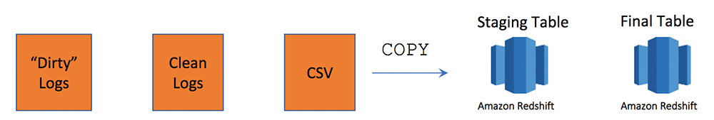
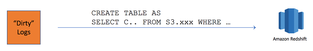
Simplifying ETL pipelines

Before Amazon Redshift Spectrum, data ingestion to Amazon Redshift could be a multistep process. A common data pipeline includes ETL processes. You need to clean dirty data, do some transformation, load the data into a staging area, then load the data to the final table. You might need to use different services for each step, and coordinate among them. The following diagram illustrates this workflow.

Using Amazon Redshift Spectrum, you can streamline the complex data engineering process by eliminating the need to load data physically into staging tables.

To do so, create an external schema or table pointing to the raw data stored in Amazon S3, or use an AWS Glue or Athena data catalog. Put your transformation logic in a SELECT query and ingest the result into Amazon Redshift. You can do this all in one single query, with no additional service needed:

CREATE TABLE <Final Amazon Redshift table> AS SELECT … FROM s3_external_schema.xxx WHERE …;
SELECT … INTO <Final Amazon Redshift table> FROM s3_external_schema.xxx 
WHERE …;

The following diagram illustrates this updated workflow.

Best practices for query performance

You can improve query performance with the following suggestions.

Improving Amazon S3 query performance with predicate pushdown

You can improve performance of queries written on S3 by using predicate pushdown. To limit the amount of data scanned, apply filters on columns that are defined as partitions.

Examining your query explain plan to verify if predicate pushdown is effective

In the following query’s explain plan, the Amazon S3 scan filter is pushed down to the Amazon Redshift Spectrum layer. Therefore, only the matching results are returned to Amazon Redshift for final processing.

EXPLAIN SELECT * FROM s3_external_schema.sales WHERE memo LIKE 'return%';
XN S3 Query Scan sales  (cost=0.00..225000000.00 rows=10000000000 width=410)
  ->  S3 Seq Scan s3_external_schema.sales location:"s3://<your-bucket>/sales" format:TEXT  (cost=0.00..125000000.00 rows=10000000000 width=410)
        Filter: ((memo)::text ~~ 'return%'::text)

On the other hand, the second query’s explain plan doesn’t have a predicate pushdown to the Amazon Redshift Spectrum layer due to ILIKE. As a result, this query is forced to bring back a huge amount of data from Amazon S3 into Amazon Redshift to filter.

EXPLAIN SELECT * FROM s3_external_schema.sales WHERE memo ILIKE 'Return%';
XN S3 Query Scan sales  (cost=0.00..225000000.00 rows=512000001 width=410)
  Filter: ((memo)::text ~~* 'Return%'::text)
  ->  S3 Seq Scan s3_external_schema.sales location:"s3://<your-bucket>/sales" format:TEXT  (cost=0.00..100000000.00 rows=10000000000 width=410)

We keep improving predicate pushdown, and plan to push down more and more SQL operations over time. For example, ILIKE is now pushed down to Amazon Redshift Spectrum in the current Amazon Redshift release.

Replace complex DISTINCT operations with GROUP BY in your queries

Amazon Redshift can automatically rewrite simple DISTINCT (single-column) queries during the planning step and push them down to Amazon Redshift Spectrum.

You must perform certain SQL operations like multiple-column DISTINCT and ORDER BY in Amazon Redshift because you can’t push them down to Amazon Redshift Spectrum. If possible, you should rewrite these queries to minimize their use, or avoid using them.

As an example, examine the following two functionally equivalent SQL statements. The first query with multiple columns uses DISTINCT:

SELECT DISTINCT l_returnflag,l_linestatus 
FROM 	s3_external_schema.LINEITEM_PART_PARQ 
WHERE 	EXTRACT(YEAR from l_shipdate::DATE) BETWEEN '<Start-Year>' AND  '<End-Year>'
ORDER BY l_returnflag, l_linestatus;

The second equivalent query uses GROUP BY:

SELECT l_returnflag,l_linestatus 
FROM 	s3_external_schema.LINEITEM_PART_PARQ 
WHERE EXTRACT(YEAR from l_shipdate::DATE) BETWEEN '<Start-Year>' AND  '<End-Year>' 
GROUP BY l_returnflag, l_linestatus 
ORDER BY l_returnflag, l_linestatus;

In the first query, you can’t push the multiple-column DISTINCT operation down to Amazon Redshift Spectrum, so a large number of rows is returned to Amazon Redshift to be sorted and de-duped. In the second query, S3 HashAggregate is pushed to the Amazon Redshift Spectrum layer, where most of the heavy lifting and aggregation occurs. You can query against the SVL_S3QUERY_SUMMARY system view for these two SQL statements (check the column s3query_returned_rows). You should see a big difference in the number of rows returned from Amazon Redshift Spectrum to Amazon Redshift.

The lesson learned is that you should replace DISTINCT with GROUP BY in your SQL statements wherever possible.

Choose the right datatype when creating external tables

AWS Glue crawlers can automatically infer schema from common files with formats that include JSON, CSV, and Apache Avro. If you choose to define schema using Create External Table syntax, choose the right datatype and length for your columns to avoid memory management overhead. For example

Choose varchar(<<appropriate_length>>) instead of varchar(max)
Choose the datatype date instead of varchar for dates

Best practices for table placement and statistics

You can improve table placement and statistics with the following suggestions.

Determining the best place to store your tables

The following guidelines can help you determine the best place to store your tables for the optimal performance.

You can access data stored in Amazon Redshift and Amazon S3 in the same query. By placing data in the right storage based on access pattern, you can achieve better performance with lower cost:

Load data in Amazon S3 and use Amazon Redshift Spectrum when your data volumes are in petabyte range and when your data is historical and less frequently accessed.
Load data into Amazon Redshift if data is hot and frequently used. Amazon Redshift supports loading from text, JSON, and AVRO, Parquet, and ORC.
Roll up complex reports on Amazon S3 data nightly to small local Amazon Redshift tables. You can combine the power of Amazon Redshift Spectrum and Amazon Redshift:
- Use the Amazon Redshift Spectrum compute power to do the heavy lifting and materialize the result.
- Use Amazon Redshift as a result cache to provide faster responses.
Use a late binding view to integrate an external table and an Amazon Redshift local table if a small part of your data is hot and the rest is cold. See the following statement:

CREATE VIEW total_sales as
SELECT … FROM sales_last_month
UNION ALL
SELECT … FROM s3_external_schema.sales_historical
WITH NO SCHEMA BINDING

Setting the table statistics (numRows) manually for Amazon S3 external tables.

The Amazon Redshift optimizer can use external table statistics to generate more robust run plans. Without statistics, a plan is generated based on heuristics with the assumption that the Amazon S3 table is relatively large. For example, see the following example plan:

explain select * from s3_external_schema.event_desc ed join s3_external_schema.event e
on e.event_cd = ed.event_cd and e.event_type_cd = ed.event_type;

XN Hash Join DS_BCAST_INNER  (cost=250000000.00..356425000500000000.00 rows=173286210788786592 width=2620)
  Hash Cond: ((("outer".event_cd)::text = ("inner".event_cd)::text) AND (("outer".event_type)::text = ("inner".event_type_cd)::text))
  ->  XN S3 Query Scan e  (cost=0.00..200000000.00 rows=10000000000 width=1556)
        ->  S3 Seq Scan s3_external_schema.event_desc e location:"s3://<your-bucket>/<xyz>/event_desc/" format:PARQUET  (cost=0.00..100000000.00 rows=10000000000 width=1556)
  ->  XN Hash  (cost=200000000.00..200000000.00 rows=10000000000 width=1064)
        ->  XN S3 Query Scan ed  (cost=0.00..200000000.00 rows=10000000000 width=1064)
              ->  S3 Seq Scan s3_external_schema.event ed location:"s3://<your-bucket>/<xyz>/event/" format:PARQUET  (cost=0.00..100000000.00 rows=10000000000 width=1064)

As you can see, the join order is not optimal. How do we fix it?

Although you can’t perform ANALYZE on external tables, you can set the table statistics (numRows) manually with a TABLE PROPERTIES clause in the CREATE EXTERNAL TABLE and ALTER TABLE command:

ALTER TABLE s3_external_schema.event SET TABLE PROPERTIES ('numRows'='122857504');
ALTER TABLE s3_external_schema.event_desc SET TABLE PROPERTIES ('numRows'=' 799');

With this piece of information, the Amazon Redshift optimizer can generate more optimal run plans and complete queries faster. See the following explain plan:

XN Hash Join DS_BCAST_INNER  (cost=19.98..12696028004.76 rows=170103196 width=2620)
  Hash Cond: ((("outer".event_cd)::text = ("inner".event_cd)::text) AND (("outer".event_type_cd)::text = ("inner".event_type)::text))
  ->  XN S3 Query Scan e  (cost=0.00..2457150.08 rows=122857504 width=1064)
        ->  S3 Seq Scan s3_external_schema.event e location:"s3://<your-bucket>/<xyz>/event/" format:PARQUET  (cost=0.00..1228575.04 rows=122857504 width=1064)
  ->  XN Hash  (cost=15.98..15.98 rows=799 width=1556)
        ->  XN S3 Query Scan ed  (cost=0.00..15.98 rows=799 width=1556)
              ->  S3 Seq Scan s3_external_schema.event_desc ed location:"s3://<your-bucket>/<xyz>/event_desc/" format:PARQUET  (cost=0.00..7.99 rows=799 width=1556)

Best practices for query cost control

As mentioned earlier in this post, partition your data wherever possible, use columnar formats like Parquet and ORC, and compress your data. By doing so, you not only improve query performance, but also reduce the query cost by reducing the amount of data your Amazon Redshift Spectrum queries scan. You can also help control your query costs with the following suggestions.

Optimizing query cost using query monitoring rules

For a nonselective join, a large amount of data needs to be read to perform the join. Doing this can incur high data transfer costs and network traffic, and result in poor performance and higher than necessary costs.

Are your queries scan-heavy, selective, or join-heavy? To monitor metrics and understand your query pattern, you can use the following query:

SELECT query, 
       Round(elapsed :: FLOAT / 1000 / 1000, 3) AS elapsed_sec, 
       aborted, 
       is_partitioned, 
       s3_scanned_rows, 
       s3query_returned_rows, 
       s3_scanned_bytes, 
       s3query_returned_bytes, 
       files, 
       max_retries, 
       Round(max_request_duration :: FLOAT / 1000 / 1000, 3) AS 
       max_request_dur_sec, 
       Round(avg_request_duration :: FLOAT / 1000 / 1000, 3) AS 
       avg_request_dur_sec, 
       Round(avg_request_parallelism, 2)                     AS 
       avg_request_parallelism 
FROM   svl_s3query_summary 
WHERE  query = <Query-ID>;

As part of this, do the following:

Check the ratio of scanned to returned data and the degree of parallelism
Check if your query can take advantage of partition pruning (see the best practice Partitioning files on frequently filtered columns)

When you know what’s going on, you can set up workload management (WLM) query monitoring rules (QMR) to stop rogue queries to avoid unexpected costs.

If you forget to add a filter or data isn’t partitioned properly, a query can accidentally scan a huge amount of data and cause high costs. To set query performance boundaries, use WLM query monitoring rules and take action when a query goes beyond those boundaries. For example, you might set a rule to abort a query when spectrum_scan_size_mb is greater than 20 TB or when spectrum_scan_row_count is greater than 1 billion.

With these and other query monitoring rules, you can terminate the query, hop the query to the next matching queue, or just log it when one or more rules are triggered. For more information, see WLM query monitoring rules.

Monitoring and controlling your Amazon Redshift Spectrum usage and costs using usage limits

In provisioned clusters, Amazon Redshift Spectrum has an additional cost. You can configure usage limits, with which you can monitor and control the usage and associated costs for Amazon Redshift Spectrum. You can create daily, weekly, and monthly usage limits and define actions that Amazon Redshift automatically takes if the limits defined by you are reached. Actions include: logging an event to a system table, alerting with an Amazon CloudWatch alarm, notifying an administrator with Amazon Simple Notification Service (Amazon SNS), and disabling further usage.

To create usage limits in the new Amazon Redshift console, choose Configure usage limit from the Actions menu for your cluster. You can create, modify, and delete usage limits programmatically by using the following AWS Command Line Interface (AWS CLI) commands:

modify-usage-limit

You can also create, modify, and delete using the following API operations:

For more information, see Manage and control your cost with Amazon Redshift Concurrency Scaling and Spectrum.

Conclusion

In this post, we provide some important best practices to improve the performance of Amazon Redshift Spectrum. Because each use case is unique, you should evaluate how you can apply these recommendations to your specific situations.

We want to acknowledge our fellow AWS colleagues Bob Strahan, Abhishek Sinha, Maor Kleider, Jenny Chen, Martin Grund, Tony Gibbs, Derek Young and Nausheen Sayed for their comments, insights, and help.

If you have any questions or suggestions, please leave your feedback in the comment section. If you need further assistance in optimizing your Amazon Redshift usage, contact your AWS account team.

About the authors

Po Hong, PhD, is a Big Data Consultant in the Global Big Data & Analytics Practice of AWS Professional Services.

Peter Dalton is a Principal Consultant in AWS Professional Services.

Matt Scaer is a Principal Data Warehousing Specialist Solution Architect, with over 20 years of data warehousing experience, with 11+ years at both AWS and Amazon.com.

Juan Yu is a Data Warehouse Specialist Solutions Architect at AWS.

Ippokratis Pandis is a Principal Software Eningeer in AWS working on Amazon Redshift and Amazon Redshift Spectrum.

Anusha Challa is a Senior Analytics Specialist Solutions Architect with Amazon Web Services.

Satish Sathiya is a Product Engineer at Amazon Redshift. He is an avid big data enthusiast who collaborates with customers around the globe to achieve success and meet their data warehousing and data lake architecture needs.