Amazon Redshift Federated Query enables you to use the analytic power of Amazon Redshift to directly query data stored in Amazon Aurora PostgreSQL and Amazon RDS for PostgreSQL databases. For more information about setting up an environment where you can try out Federated Query, see Accelerate Amazon Redshift Federated Query adoption with AWS CloudFormation.
Federated Query enables real-time data integration and simplified ETL processing. You can now connect live data sources directly in Amazon Redshift to provide real-time reporting and analysis. Previously, you needed to extract data from your PostgreSQL database to Amazon Simple Storage Service (Amazon S3) and load it to Amazon Redshift using COPY or query it from Amazon S3 with Amazon Redshift Spectrum. For more information about the benefits of Federated Query, see Build a Simplified ETL and Live Data Query Solution using Amazon Redshift Federated Query.
This post discusses 10 best practices to help you maximize the benefits of Federated Query when you have large federated data sets, when your federated queries retrieve large volumes of data, or when you have many Redshift users accessing federated data sets. These techniques are not necessary for general usage of Federated Query. They are intended for advanced users who want to make the most of this exciting feature.
The best practices are divided into two sections: the first for advice that applies to your Amazon Redshift cluster, and the second for advice that applies to your Aurora PostgreSQL and Amazon RDS for PostgreSQL environments.
The code examples provided in this post derive from the data and queries in the CloudDataWarehouseBenchmark GitHub repo (based on TPC-H and TPC-DS).
Best practices to apply in Amazon Redshift
The following best practices apply to your Amazon Redshift cluster when using federated queries to access your Aurora or Amazon RDS for PostgreSQL instances.
1. Use separate external schemas for each use case
Consider creating separate Amazon Redshift external schemas, using separate remote PostgreSQL users, for each specific Amazon Redshift use case. This practice allows you to have extra control over the users and groups who can access the external database. For instance, you may want to have an external schema for ETL usage, with an associated PostgreSQL user, that has broad access and another schema, and an associated PostgreSQL user for ad-hoc reporting and analysis with access limited to specific resources.
The following code example creates two external schemas for ETL use and ad-hoc reporting use. Each schema uses a different SECRET_ARN containing credentials for separate users in the PostgreSQL database.
-- ETL usage - broad access
CREATE EXTERNAL SCHEMA IF NOT EXISTS apg_etl
FROM POSTGRES DATABASE 'tpch' SCHEMA 'public'
URI 'aurora-postgres-ro.cr7d8lhiupkf.us-west-2.rds.amazonaws.com' PORT 8192
IAM_ROLE 'arn:aws:iam::123456789012:role/apg-federation-role'
SECRET_ARN 'arn:aws:secretsmanager:us-west-2:123456789012:secret:apg-redshift-etl-secret-187Asd'
;
-- Ad-Hoc usage - limited access
CREATE EXTERNAL SCHEMA IF NOT EXISTS apg_adhoc
FROM POSTGRES DATABASE 'tpch' SCHEMA 'public'
URI 'aurora-postgres-ro.cr7d8lhiupkf.us-west-2.rds.amazonaws.com' PORT 8192
IAM_ROLE 'arn:aws:iam::123456789012:role/apg-federation-role'
SECRET_ARN 'arn:aws:secretsmanager:us-west-2:123456789012:secret:apg-redshift-adhoc-secret-187Asd'
;
2. Use query timeouts to limit total runtimes
Consider setting a timeout on the users or groups that have access to your external schemas. User queries could unintentionally try to retrieve a very large number of rows from the external relation and remain running for an extended time, which holds open resources in both Amazon Redshift and PostgreSQL.
To limit the total runtime of a user’s queries, you can set a statement_timeout for all a user’s queries. The following code example sets a 2-hour timeout for an ETL user:
-- Set ETL user timeout to 2 hours
ALTER USER etl_user SET statement_timeout TO 7200000;
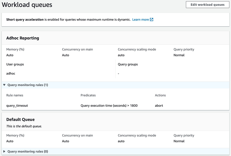
If many users have access to your external schemas, it may not be practical to define a statement_timeout for each individual user. Instead, you can add a query monitoring rule in your WLM configuration using the query_execution_time metric. The following screenshot shows an Auto WLM configuration with an Adhoc Reporting queue for users in the adhoc group, with a rule that cancels queries that run for longer than 1,800 seconds (30 minutes).
3. Make sure the Amazon Redshift query plan is efficient
Review the overall query plan and query metrics of your federated queries to make sure that Amazon Redshift processes them efficiently. For more information about query plans, see Evaluating the query plan.
Viewing the Amazon Redshift query explain plan
You can retrieve the plan for your query by prefixing your SQL with EXPLAIN and running that in your SQL client. The following code example is the explain output for a sample query:
<< REDSHIFT >> QUERY PLAN
-------------------------------------------------------------------------------------------------------------
 XN Aggregate  (cost=6396670427721.37..6396670427721.37 rows=1 width=32)
   ->  XN Hash Join DS_BCAST_INNER  (cost=499986.50..6396670410690.30 rows=6812425 width=32)
         Hash Cond: ("outer".l_partkey = ("inner".p_partkey)::bigint)
         ->  XN Seq Scan on lineitem  (cost=0.00..2997629.29 rows=199841953 width=40)
               Filter: ((l_shipdate < '1994-03-01'::date) AND (l_shipdate >= '1994-02-01'::date))
         ->  XN Hash  (cost=449987.85..449987.85 rows=19999460 width=4)
               ->  XN PG Query Scan part  (cost=0.00..449987.85 rows=19999460 width=4)
                     ->  Remote PG Seq Scan apg_tpch_100g.part  (cost=0.00..249993.25 rows=19999460 width=4)
                           Filter: ((p_type)::text ~~ 'PROMO%'::text)
The operator XN PG Query Scan indicates that Amazon Redshift will run a query against the federated PostgreSQL database for this part of the query, we refer to this as the “federated subquery” in this post. When your query uses multiple federated data sources Amazon Redshift runs a federated subquery for each source. Amazon Redshift runs each federated subquery from a randomly selected node in the cluster.
Below the XN PG Query Scan line, you can see Remote PG Seq Scan followed by a line with a Filter: element. These two lines define how Amazon Redshift accesses the external data and the predicate used in the federated subquery. You can see that the federated subquery will run against the federated table apg_tpch.part.
You can also see from rows=19999460 that Amazon Redshift estimates that the query can return up to 20 million rows from PostgreSQL. It creates this estimate by asking PostgreSQL for statistics about the table.
Joins
Since each federated subquery runs from a single node in the cluster, Amazon Redshift must choose a join distribution strategy to send the rows returned from the federated subquery to the rest of the cluster to complete the joins in your query. The choice of a broadcast or distribution strategy is indicated in the explain plan. Operators that start with DS_BCAST broadcast a full copy of the data to all nodes. Operators that start with DS_DIST distribute a portion of the data to each node in the cluster.
It’s usually most efficient to broadcast small results and distribute larger results. When the planner has a good estimate of the number of rows that the federated subquery will return, it chooses the correct join distribution strategy. However, if the planner’s estimate isn’t accurate, it may choose broadcast for result that is too large, which can slow down your query.
Join Order
Joins should use the smaller result as the inner relation. When your query joins two tables (or two federated subqueries), Amazon Redshift must choose how best to perform the join. The query planner may not perform joins in the order declared in your query. Instead, it uses the information it has about the relations being joined to create estimated costs for a variety of possible plans. It uses the plan, including join order, that has the lowest expected cost.
When you use a hash join, the most common join, Amazon Redshift constructs a hash table from the inner table (or result) and compares it to every row from the outer table. You want to use the smallest result as the inner so that the hash table can fit in memory. The chosen ordering join may not be optimal if the planner’s estimate doesn’t reflect the real size of the results from each step in the query.
Improving query efficiency
The following is high-level advice for improving efficiency. For more information, see Analyzing the query plan.
- Examine the plan for separate parts of your query. If your query has multiple joins or uses subqueries, you can review the explain plan for each join or subquery to check whether the query benefits from being simplified. For instance, if you use several joins, examine the plan for a simpler query using only one join to see how Amazon Redshift plans that join on its own.
- Examine the order of outer joins and use an inner join. The planner can’t always reorder outer joins. If you can convert an outer join to an inner join, it may allow the planner to use a more efficient plan.
- Reference the distribution key of the largest Amazon Redshift table in the join. When a join references the distribution key Amazon Redshift can complete the join on each node in parallel without moving the rows from the Redshift table across the cluster.
- Insert the federated subquery result into a table. Amazon Redshift has optimal statistics when the data comes from a local temporary or permanent table. In rare cases, it may be most efficient to store the federated data in a temporary table first and join it with your Amazon Redshift data.
4. Make sure predicates are pushed down to the remote query
Amazon Redshift’s query optimizer is very effective at pushing predicate conditions down to the federated subquery that runs in PostgreSQL. Review the query plan of important or long-running federated queries to check that Amazon Redshift applies all applicable predicates to each subquery.
Consider the following example query, in which the predicate is inside a CASE statement and the federated relation is within a CTE subquery:
WITH cte
AS (SELECT p_type, l_extendedprice, l_discount, l_quantity
    FROM public.lineitem
    JOIN apg_tpch.part --<< PostgreSQL table
         ON l_partkey = p_partkey
    WHERE l_shipdate >= DATE '1994-02-01'
      AND l_shipdate < (DATE '1994-02-01' + INTERVAL '1 month')
)
SELECT CASE WHEN p_type LIKE 'PROMO%' --<< PostgreSQL filter predicate pt1
            THEN TRUE ELSE FALSE END AS is_promo
     , AVG( ( l_extendedprice * l_discount) / l_quantity ) AS avg_promo_disc_val
FROM cte
WHERE is_promo IS TRUE --<< PostgreSQL filter predicate pt2
GROUP BY 1;
Amazon Redshift can still effectively optimize the federated subquery by pushing a filter down to the remote relation. See the following plan:
<< REDSHIFT >> QUERY PLAN
-------------------------------------------------------------------------------------------------------------------
 XN HashAggregate  (cost=17596843176454.83..17596843176456.83 rows=200 width=87)
   ->  XN Hash Join DS_BCAST_INNER  (cost=500000.00..17596843142391.79 rows=6812609 width=87)
         Hash Cond: ("outer".l_partkey = ("inner".p_partkey)::bigint)
         ->  XN Seq Scan on lineitem  (cost=0.00..2997629.29 rows=199841953 width=40)
               Filter: ((l_shipdate < '1994-03-01'::date) AND (l_shipdate >= '1994-02-01'::date))
         ->  XN Hash  (cost=450000.00..450000.00 rows=20000000 width=59)-- Federated subquery >>
               ->  XN PG Query Scan part  (cost=0.00..450000.00 rows=20000000 width=59)
                     ->  Remote PG Seq Scan apg_tpch.part  (cost=0.00..250000.00 rows=20000000 width=59)
                           Filter: (CASE WHEN ((p_type)::text ~~ 'PROMO%'::text) THEN true ELSE false END IS TRUE)-- << Federated subquery
If Redshift can’t push your predicates down as needed, or the query still returns too much data, consider the advice in the following two sections regarding materialized views and syncing tables. To easily rewrite your queries to achieve effective filter pushdown, consider the advice in the final best practice regarding persisting frequently queried data.
5. Use materialized views to cache frequently accessed data
Amazon Redshift now supports the creation of materialized views that reference federated tables in external schemas.
Cache queries that run often
Consider caching frequently run queries in your Amazon Redshift cluster using a materialized view. When many users run the same federated query regularly, the remote content of the query must be retrieved again for each execution. With a materialized view, the results can instead be retrieved from your Amazon Redshift cluster without getting the same data from the remote database. You can then schedule the refresh of the materialized view to happen at a specific time, depending upon the change rate and importance of the remote data.
The following code example demonstrates the creation, querying, and refresh of a materialized view from a query that uses a federated source table:
-- Create the materialized view
CREATE MATERIALIZED VIEW mv_store_quantities_by_quarter AS
SELECT ss_store_sk
     , d_quarter_name
     , COUNT(ss_quantity) AS count_quantity
     , AVG(ss_quantity) AS avg_quantity
FROM public.store_sales
JOIN apg_tpcds.date_dim --<< federated table
    ON d_date_sk = ss_sold_date_sk
GROUP BY ss_store_sk
ORDER BY ss_store_sk
;
--Query the materialized view
SELECT *
FROM mv_store_quanties_by_quarter
WHERE d_quarter_name = '1998Q1'
;
--Refresh the materialized view
REFRESH MATERIALIZED VIEW mv_store_quanties_by_quarter
;
Cache tables that are used by many queries
Also consider locally caching tables used by many queries using a materialized view. When many different queries use the same federated table it’s often better to create a materialized view for that federated table which can then be referenced by the other queries instead.
The following code example demonstrates the creation and querying of a materialized view on a single federated source table:
-- Create the materialized view
CREATE MATERIALIZED VIEW mv_apg_part AS
SELECT * FROM apg_tpch_100g.part
;
--Query the materialized view
SELECT SUM(l_extendedprice * (1 - l_discount)) AS discounted_price
FROM public.lineitem, mv_apg_part
WHERE l_partkey = p_partkey
  AND l_shipdate BETWEEN '1997-03-01' AND '1997-04-01'
;
As of this writing, you can’t reference a materialized view inside another materialized view. Other views that use the cached table need to be regular views.
Balance caching against refresh time and frequency
The use of materialized views is best suited for queries that run quickly relative to the refresh schedule. For example, a materialized view refreshed hourly should run in a few minutes, and a materialized view refreshed daily should run in less than an hour. As of this writing, materialized views that reference external tables aren’t eligible for incremental refresh. A full refresh occurs when you run REFRESH MATERIALIZED VIEW and recreate the entire result.
Limit remote access using materialized views
Also consider using materialized views to reduce the number of users who can issue queries directly against your remote databases. You can grant external schema access only to a user who refreshes the materialized views and grant other Amazon Redshift users access only to the materialized view.
Limiting the scope of access in this way is a general best practice for data security when querying from remote production databases that contain sensitive information.
6. Sync large remote tables to a local copy
Consider keeping a copy of the remote table in a permanent Amazon Redshift table. When your remote table is large and a full refresh of a materialized view is time-consuming it’s more effective to use a sync process to keep a local copy updated.
Sync newly added remote data
When your large remote table only has new rows added, not updated nor deleted, you can synchronize your Amazon Redshift copy by periodically inserting the new rows from the remote table into the copy. You can automate this sync process using the example stored procedure sp_sync_get_new_rows on GitHub.
This example stored procedure requires the source table to have an auto-incrementing identity column as its primary key. It finds the current maximum in your Amazon Redshift table, retrieves all rows in the federated table with a higher ID value, and inserts them into the Amazon Redshift table.
The following code examples demonstrate a sync from a federated source table to a Amazon Redshift target table. First, you create a source table with four rows in the PostgreSQL database:
CREATE TABLE public.pg_source (
      pk_col   BIGINT GENERATED ALWAYS AS IDENTITY PRIMARY KEY
    , data_col VARCHAR(20));
INSERT INTO public.pg_tbl (data_col)
VALUES ('aardvark'),('aardvarks'),('aardwolf'),('aardwolves')
;
Create a target table with two rows in your Amazon Redshift cluster:
CREATE TABLE public.rs_target (
      pk_col   BIGINT PRIMARY KEY
    , data_col VARCHAR(20));
INSERT INTO public.rs_tbl
VALUES (1,'aardvark'), (2,'aardvarks')
;
Call the Amazon Redshift stored procedure to sync the tables:
CALL sp_sync_get_new_rows(SYSDATE,'apg_tpch.pg_source','public.rs_target','pk_col','public.sp_logs',0);
-- INFO:  SUCCESS - 2 new rows inserted into `target_table`.

SELECT * FROM public.rs_tbl;
--  pk_col |  data_col
-- --------+------------
--       1 | aardvark
--       2 | aardvarks
--       4 | aardwolves
--       3 | aardwolf
Merge remote data changes
After you update or insert rows in your remote table, you can synchronize your Amazon Redshift copy by periodically merging the changed rows and new rows from the remote table into the copy. This approach works best when changes are clearly marked in the table so that you can easily retrieve just the new or changed rows. You can automate this sync process using the example stored procedure sp_sync_merge_changes, on GitHub.
This example stored procedure requires the source to have a date/time column that indicates the last time each row was modified. It uses this column to find changes that you need to sync and either updates the changed rows or inserts new rows in the Amazon Redshift copy. The stored procedure also requires the table to have a primary key declared. It uses the primary key to identify which rows to update in the local copy of the data.
The following code examples demonstrate a refresh from a federated source table to an Amazon Redshift target table. First, create a sample table with two rows in your Amazon Redshift cluster:
CREATE TABLE public.rs_tbl (
      pk_col   INTEGER PRIMARY KEY
    , data_col VARCHAR(20)
    , last_mod TIMESTAMP);
INSERT INTO public.rs_tbl
VALUES (1,'aardvark', SYSDATE), (2,'aardvarks', SYSDATE);

SELECT * FROM public.rs_tbl;
--  pk_col |  data_col  |     last_mod
-- --------+------------+---------------------
--       1 | aardvark   | 2020-04-01 18:01:02
--       2 | aardvarks  | 2020-04-01 18:01:02
Create a source table with four rows in your PostgreSQL database:
CREATE TABLE public.pg_tbl (` `
      pk_col   INTEGER GENERATED ALWAYS AS IDENTITY PRIMARY KEY
    , data_col VARCHAR(20)
    , last_mod TIMESTAMP);
INSERT INTO public.pg_tbl (data_col, last_mod)
VALUES ('aardvark', NOW()),('aardvarks', NOW()),('aardwolf', NOW()),('aardwolves', NOW());
Call the Amazon Redshift stored procedure to sync the tables:
CALL sp_sync_merge_changes(SYSDATE,'apg_tpch.pg_tbl','public.rs_tbl','last_mod','public.sp_logs',0);
-- INFO:  SUCCESS - 4 rows synced.

SELECT * FROM public.rs_tbl;
--  pk_col |  data_col  |      last_mod
-- --------+------------+---------------------
--       1 | aardvark   | 2020-04-01 18:09:56
--       2 | aardvarks  | 2020-04-01 18:09:56
--       4 | aardwolves | 2020-04-01 18:09:56
--       3 | aardwolf   | 2020-04-01 18:09:56
Best practices to apply in Aurora or Amazon RDS
The following best practices apply to your Aurora or Amazon RDS for PostgreSQL instances when using them with Amazon Redshift federated queries.
7. Use a read replica to minimize Aurora or RDS impact
Aurora and Amazon RDS allow you to configure one or more read replicas of your PostgreSQL instance. As of this writing, Federated Query doesn’t allow writing to the federated database, so you should use a read-only endpoint as the target for your external schema. This also makes sure that the federated subqueries Amazon Redshift issues have the minimum possible impact on the master database instance, which often runs a large number of small and fast write transactions.
For more information about read replicas, see Adding Aurora Replicas to a DB Cluster and Working with PostgreSQL Read Replicas in Amazon RDS.
The following code example creates an external schema using a read-only endpoint. You can see the -ro naming in the endpoint URI configuration:
--In Amazon Redshift:
CREATE EXTERNAL SCHEMA IF NOT EXISTS apg_etl
FROM POSTGRES DATABASE 'tpch' SCHEMA 'public'
URI 'aurora-postgres-ro.cr7d8lhiupkf.us-west-2.rds.amazonaws.com' PORT 8192
IAM_ROLE 'arn:aws:iam::123456789012:role/apg-federation-role'
SECRET_ARN 'arn:aws:secretsmanager:us-west-2:123456789012:secret:apg-redshift-etl-secret-187Asd';
8. Use specific and limited PostgreSQL users for each use case
As mentioned in the first best practice regarding separate external schemas, consider creating separate PostgreSQL users for each federated query use case. Having multiple users allows you to grant only the permissions needed for each specific use case. Each user needs a different SECRET_ARN, containing its access credentials, for the Amazon Redshift external schema to use. See the following code:
-- Create an ETL user who will have broad access
CREATE USER redshift_etl WITH PASSWORD '<<example>>';
-- Create an Ad-Hoc user who will have limited access
CREATE USER redshift_adhoc WITH PASSWORD '<<example>>';
Apply a user timeout to limit query runtime
Consider setting a statement_timeout on your PostgreSQL users. A user query could accidentally try to retrieve many millions of rows from the external relation and remain running for an extended time, which holds open resources in both Amazon Redshift and PostgreSQL. To prevent this, specify different timeout values for each user according to their expected usage. The following code example sets timeouts for an ETL user and an ad-hoc reporting user:
-- Set ETL user timeout to 1 hour
ALTER USER redshift_etl SET statement_timeout TO 3600000;
-- Set Ad-Hoc user timeout to 15 minutes
ALTER USER redshift_adhoc SET statement_timeout TO 900000;
9. Make sure the PostgreSQL table is correctly indexed
Consider adding or modifying PostgreSQL indexes to make sure Amazon Redshift federated queries run efficiently. Amazon Redshift retrieves data from PostgreSQL using regular SQL queries against your remote database. Queries are often faster when using an index, particularly when the query returns a small portion of the table.
Consider the following code example of an Amazon Redshift federated query on the lineitem table:
SELECT AVG( ( l_extendedprice * l_discount) / l_quantity ) AS avg_disc_val
FROM apg_tpch.lineitem
WHERE l_shipdate >= DATE '1994-02-01'
  AND l_shipdate < (DATE '1994-02-01' + INTERVAL '1 day');
Amazon Redshift rewrites this into the following federated subquery to run in PostgreSQL:
SELECT pg_catalog."numeric"(l_discount)
     , pg_catalog."numeric"(l_extendedprice)
     , pg_catalog."numeric"(l_quantity)
FROM public.lineitem
WHERE (l_shipdate < '1994-02-02'::date)
  AND (l_shipdate >= '1994-02-01'::date);
Without an index, you get the following plan from PostgreSQL:
<< POSTGRESQL >> QUERY PLAN [No Index]
--------------------------------------------------------------------------------------------
 Gather  (cost=1000.00..16223550.40 rows=232856 width=17)
   Workers Planned: 2
   ->  Parallel Seq Scan on lineitem  (cost=0.00..16199264.80 rows=97023 width=17)
         Filter: ((l_shipdate < '1994-02-02'::date) AND (l_shipdate >= '1994-02-01'::date))
You can add the following index to cover exactly the data this query needs:
CREATE INDEX lineitem_ix_covering
ON public.lineitem (l_shipdate, l_extendedprice, l_discount, l_quantity);
With the new index in place, you see the following plan:
<< POSTGRESQL >> QUERY PLAN [With Covering Index]
------------------------------------------------------------------------------------------------
 Bitmap Heap Scan on lineitem  (cost=7007.35..839080.74 rows=232856 width=17)
   Recheck Cond: ((l_shipdate < '1994-02-02'::date) AND (l_shipdate >= '1994-02-01'::date))
   ->  Bitmap Index Scan on lineitem_ix_covering  (cost=0.00..6949.13 rows=232856 width=0)
         Index Cond: ((l_shipdate < '1994-02-02'::date) AND (l_shipdate >= '1994-02-01'::date))
In the revised plan, the max cost is 839080 versus the original 16223550—19 times less. The reduced cost suggests that the query is faster when using the index, but testing is needed to confirm this.
Indexes require careful consideration. The detailed tradeoffs of adding additional indexes in PostgreSQL, the specific PostgreSQL index types available, and index usage techniques are beyond the scope of this post.
10. Replace restrictive joins with a remote view
Many analytic queries use joins to restrict the rows that the query returns. For instance, you might apply a predicate such as calender_quarter='2019Q4' to your date_dim table and join to your large fact table. The filter on date_dim reduces the rows returned from the fact table by an order of magnitude. However, as of this writing, Amazon Redshift can’t push such join restrictions down to the federated relation.
Consider the following example query with a join between two federated tables:
SELECT ss_store_sk
,COUNT(ss_quantity) AS count_quantity
,AVG(ss_quantity) AS avg_quantity
FROM apg_tpcds.store_sales
JOIN apg_tpcds.date_dim
  ON d_date_sk = ss_sold_date_sk
WHERE d_quarter_name = '1998Q1'
GROUP BY ss_store_sk
ORDER BY ss_store_sk
LIMIT 100;
When you EXPLAIN this query in Amazon Redshift, you see the following plan:
<< REDSHIFT >> QUERY PLAN [Original]
----------------------------------------------------------------------------------------------------------------------------------
<< snip >>
  ->  XN PG Query Scan store_sales  (cost=0.00..576019.84 rows=28800992 width=12)
        ->  Remote PG Seq Scan store_sales  (cost=0.00..288009.92 rows=28800992 width=12)
  ->  XN Hash  (cost=1643.60..1643.60 rows=73049 width=4)
        ->  XN PG Query Scan date_dim  (cost=0.00..1643.60 rows=73049 width=4)
              ->  Remote PG Seq Scan date_dim  (cost=0.00..913.11 rows=73049 width=4)
                    Filter: (d_quarter_name = '1998Q1'::bpchar)
The query plan shows that date_dim is filtered, but store_sales doesn’t have a filter. This means Amazon Redshift retrieves all rows from store_sales and only then uses the join to filter the rows. Because store_sales is a very big table, this probably takes too long, especially if you want to run this query regularly.
As a solution, you can create the following view in PostgreSQL that encapsulates this join:
CREATE VIEW vw_store_sales_quarter
AS SELECT ss.*, dd.d_quarter_name ss_quarter_name
FROM store_sales   ss
JOIN date_dim      dd
    ON ss.ss_sold_date_sk = dd.d_date_sk;
Rewrite the Amazon Redshift query to use the view as follows:
SELECT ss_store_sk
      ,COUNT(ss_quantity) AS count_quantity
      ,AVG(ss_quantity) AS avg_quantity
FROM apg_tpcds_10g.vw_store_sales_date
WHERE ss_quarter_name = '1998Q1'
GROUP BY ss_store_sk
ORDER BY ss_store_sk
LIMIT 100;
When you EXPLAIN this rewritten query in Amazon Redshift, you see the following plan:
<< REDSHIFT >> QUERY PLAN [Remote View]
----------------------------------------------------------------------------------------------------------------------------------
<< snip >>
  ->  XN HashAggregate  (cost=30.00..31.00 rows=200 width=8)
        ->  XN PG Query Scan vw_store_sales_date  (cost=0.00..22.50 rows=1000 width=8)
              ->  Remote PG Seq Scan vw_store_sales_date  (cost=0.00..12.50 rows=1000 width=8)
                    Filter: (ss_quarter_name = '1998Q1'::bpchar)
Amazon Redshift now pushes the filter down to your view. The join restriction is applied in PostgreSQL and many fewer rows are returned to Amazon Redshift. You may notice that Remote PG Seq Scan now shows rows=1000; this is a default value that the query optimizer uses when PostgreSQL can’t provide table statistics.
Summary
This post reviewed 10 best practices to help you maximize the performance Amazon Redshift federated queries. Every use case is unique, so carefully evaluate how you can apply these recommendations to your specific situation.
AWS will continue to enhance and improve Amazon Redshift Federated Query, and welcomes your feedback. If you have any questions or suggestions, leave your feedback in the comments. If you need further assistance in optimizing your Amazon Redshift cluster, contact your AWS account team.
Special thanks go to AWS colleagues Sriram Krishnamurthy, Entong Shen, Niranjan Kamat, Vuk Ercegovac, and Ippokratis Pandis for their help and support with this post.
About the Author
 Joe Harris is a senior Redshift database engineer at AWS, focusing on Redshift performance. He has been analyzing data and building data warehouses on a wide variety of platforms for two decades. Before joining AWS he was a Redshift customer from launch day in 2013 and was the top contributor to the Redshift forum.