AWS Big Data Blog
Analyze and visualize nested JSON data with Amazon Athena and Amazon QuickSight
April 2024: This post was reviewed for accuracy.
Although structured data remains the backbone for many data platforms, increasingly unstructured or semi-structured data is used to enrich existing information or create new insights. Amazon Athena enables you to analyze a wide variety of data. This includes tabular data in CSV or Apache Parquet files, data extracted from log files using regular expressions, and JSON-formatted data. Athena is serverless, so there is no infrastructure to manage, and you pay only for the queries that you run.
In this post, we show you how to use JSON-formatted data and translate a nested data structure into a tabular view. For data engineers, using this type of data is becoming increasingly important. For example, you can use API-powered data feeds from operational systems to create data products. Such data can also help add more fine-grained facets to your understanding of customers and interactions. Understanding the fuller picture helps you better understand your customers and tailor experiences or predict outcomes.
Solution overview
To illustrate, we use an end-to-end example. It processes financial data stored in an Amazon Simple Storage Service (Amazon S3) bucket that is formatted as JSON. We analyze the data in Athena and visualize the results in Amazon QuickSight. Along the way, we compare and contrast alternative options.
The result looks similar to the following visualization.

Analyze JSON-formatted data
Our end-to-end example is inspired by a real-word use case, but for simplicity we use fictional generated data for this post. The data contains daily stock quote values of 10 reported years of a stock.
The following code shows example output. On the top level is an attribute called symbol, which identifies the stock described here: the fictional entity Wild Rydes fruits (WILDRYDESFRUITS). On the same level is an attribute called financials. This is a data container. The actual information is one level below, including such attributes as high, low, lastClose, and volume.
The data container is an array, where every element represents data on a given date (reportDate). In the example following, financial data for only one day is shown. However, the {...} indicates that there might be more. In our case, data for previous years is stored in the object on a daily granularity.
It has become commonplace to use external data from API operations, frequently formatted as JSON, and then to feed them into Amazon S3. This is usually done in an automated fashion. For our post, we generated synthetic data in a typical API response format.
To download the data, you can use the AWS Command Line Interface (AWS CLI) or Amazon S3 API. The following code is an example of using the AWS CLI from a terminal session:
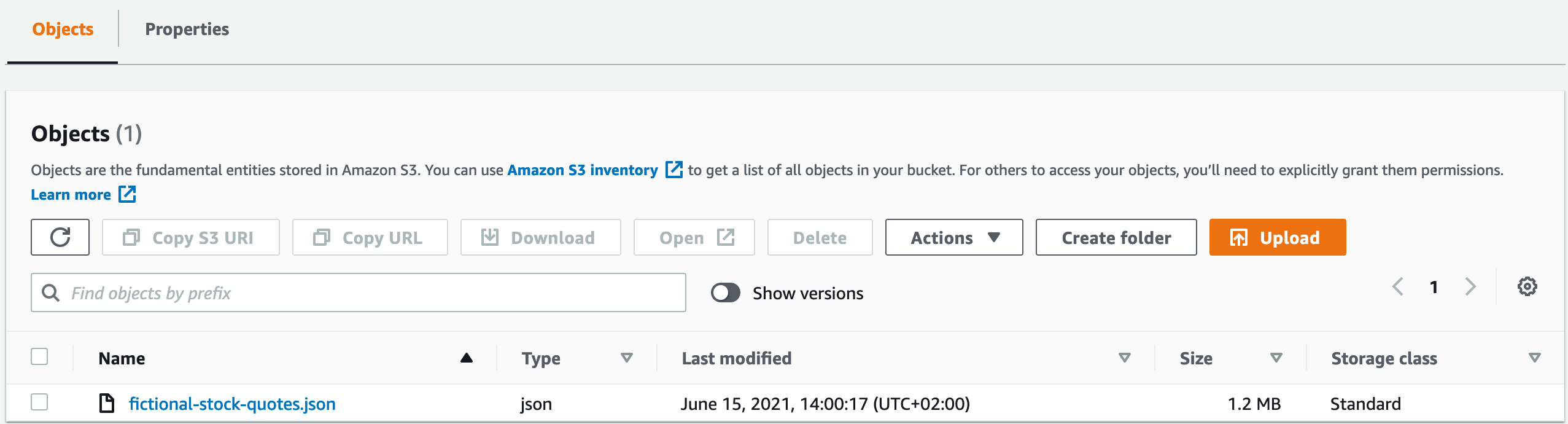
Alternatively, you can access fictional-stock-quotes.json directly. You can save the resulting JSON files to your local disk, then upload the JSON to an S3 bucket. In my case, the location of the data is s3://athena-json/financials, but you should create your own bucket. The result looks similar to the following screenshot.
Alternatively, you can use AWS CloudShell, a local shell, your local computer, or an Amazon Elastic Compute Cloud (Amazon EC2) instance to populate an Amazon S3 location with the API data:
Map JSON structures to table structures
Now we have the data in Amazon S3. Let’s make it accessible to Athena. This is a simple two-step process:
- Create metadata. Doing so is analogous to traditional databases, where we use DDL to describe a table structure. This step maps the structure of the JSON-formatted data to columns.
- Specify where to find the JSON files.
We can use all the information of the JSON file at this time, or we can concentrate on mapping the information that we need today. The new data structure in Athena overlays the files in Amazon S3 only virtually. Therefore, even though we just map a subset of the contained information at this time, all information is retained in the files and can be used later on as needed. This is a powerful concept and enables an iterative approach to data modeling.
You can use the following SQL statement to create the table. The table is then named financials_raw (see (1) in the following code). We use that name to access the data from this point on. We map the symbol and the list of financials as an array and some figures. We define that the underlying files are to be interpreted as JSON in (2), and that the data lives in s3://athena-json/financials/ in (3).
You can run this statement via the Athena console, as depicted in the following screenshot.

After you run the SQL statement, the newly created table financials_raw is listed under the heading Tables. Now let’s look what’s in this table. Choose the three vertical dots to the right of the table name and choose Preview table. Athena creates a SELECT statement to show 10 rows of the table.
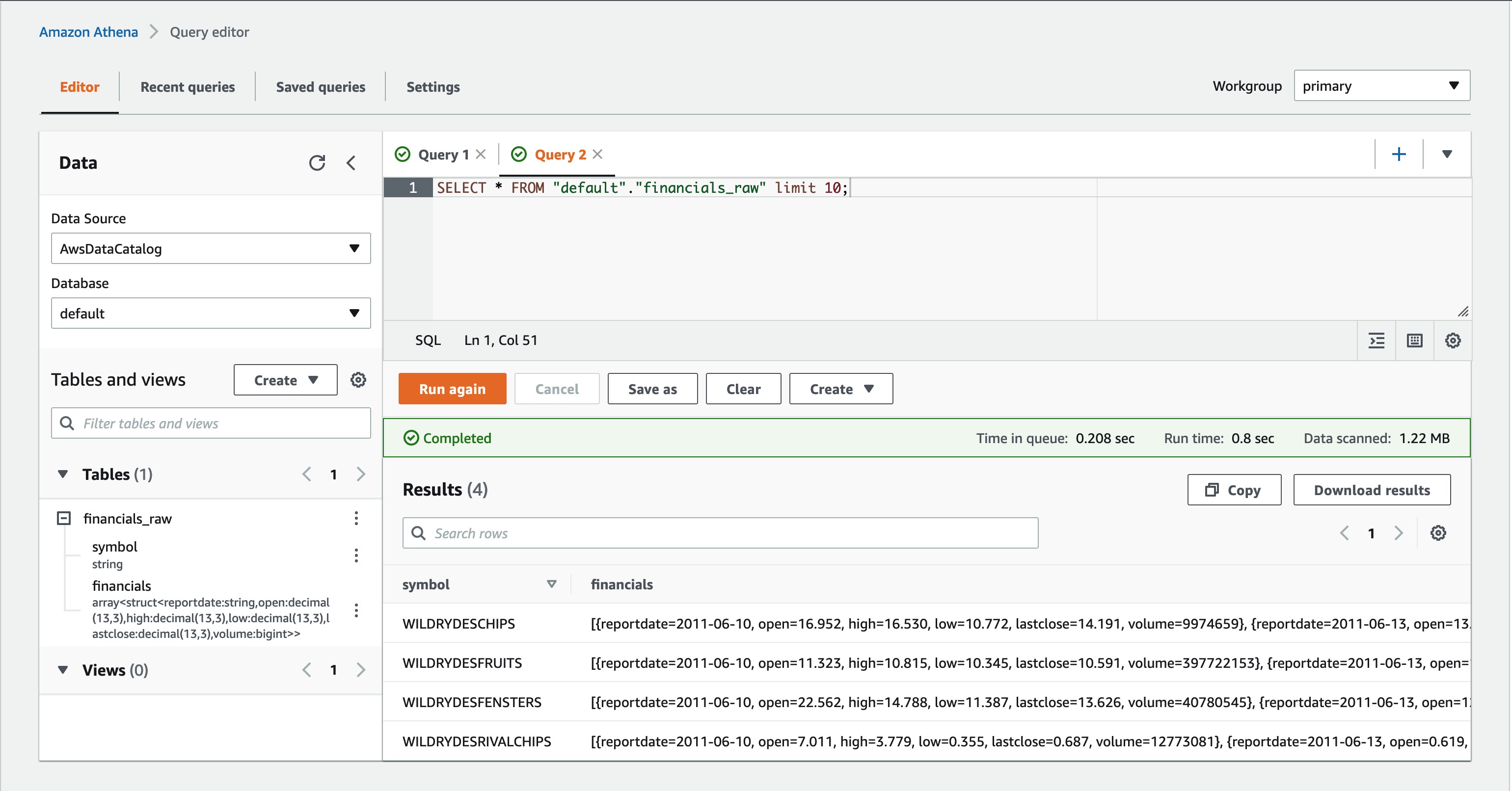
Looking at the output, you can see that Athena was able to understand the underlying data in the JSON files. Specifically, we can see two columns:
- symbol – Contains flat data, the symbol of the stock
- financials – Contains an array of financial reports
If you look closely and observe the reportdate attribute, you find that the row contains more than one financial report.
Even though the data is nested—in our case financials is an array—you can access the elements directly from your column projections:
As the following screenshot shows, all data is accessible. From this point on, it is structured, nested data, but not JSON anymore.

It’s still not tabular, though. We come back to this later in the post. First, let’s look at a different way that would also have brought us to this point.
Alternative approach: Defer the JSON extraction to query time
There are many different ways to use JSON-formatted data in Athena. In the previous section, we use a simple, explicit, and rigid approach. In contrast, we now see a rather generic, dynamic approach.
In this case, we defer the final decisions about the data structures from table design to query design. To do that, we leave the data untouched in its JSON form as long as possible. As a consequence, the CREATE TABLE statement is much simpler than in the previous section:
We run a SELECT query to preview the table:
The following screenshot shows that the data is accessible.
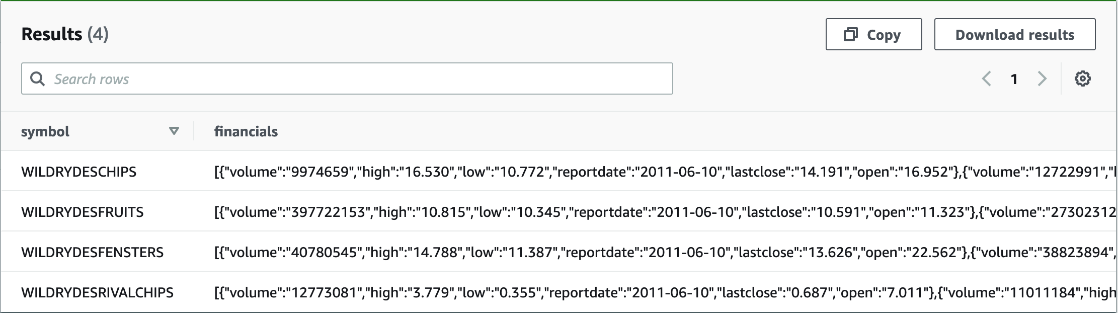
Even though the data is now accessible, it’s only treated as a single string or VARCHAR. This type is generic and doesn’t reflect the rich structure and the attributes of the underlying data.
Before diving into the richness of the data, I want to acknowledge that it’s hard to see from the query results which data type a column is. When using your queries, the focus is on the actual data, so seeing the data types all the time can be distracting. However, in this case, when creating your queries and data structures, it’s useful to use typeof. For example, use the following SQL statement:
With this SQL statement, you can verify that the column is treated as a VARCHAR.
For more information about the data structure during query design, see Querying JSON.
The following table shows how to extract the data, starting at the root of the record in the first example. The table includes additional examples on how to navigate further down the document tree. The first column shows the expression that you can use in a SQL statement like SELECT <expr> FROM financials_raw_json, where <expr> is replaced by the expression in the first column. The remaining columns explain the results.
| Expression | Result | Type | Description |
|---|---|---|---|
json_extract(financials, '$') |
[{.., "reportdate":"2017-12-31",..},{..}, {..}, {.., "reportdate":"2014-12-31", ..}] |
JSON | Selecting the root of the document (financials). |
json_extract(financials, '$[0]') |
{.., "reportdate":"2021-06-09", "volume":"17937632", ..} |
JSON | Selecting the first element of the financials array. The indexing starts at 0, as opposed to 1, which is customary in SQL. |
json_extract(financials, '$[0].reportdate') |
"2017-12-31" |
JSON | Selecting the reportdate attribute of the first element of the financials array. |
json_extract_scalar(financials, '$[0].reportdate') |
2017-12-31 |
VARCHAR | As preceding, but now the type became a VARCHAR because we’re using json_extract_scalar. |
json_size(financials, '$') |
2516 |
BIGINT | The size of the financials array; 4 represents the 4 years contained in each JSON. |
We now have more than enough understanding to implement our example.
However, there are more functions to go back and forth between JSON and Athena. For more information, see JSON Functions and Operators. Athena is our managed service based on Apache Presto. Therefore, when looking for information, it’s also helpful to consult Presto documentation.
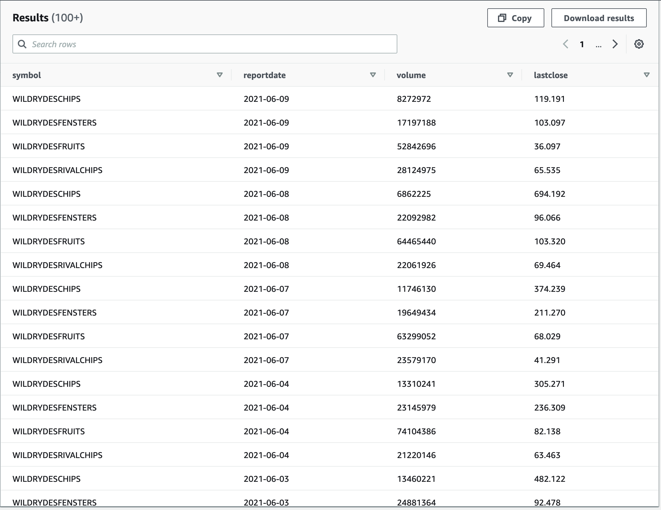
Let’s put the JSON functions we introduced earlier to use:
The following screenshot shows our results.

As with the first approach, we still have to deal with the nested data inside the rows. By doing so, we can get rid of the explicit indexing of the financial reports as used earlier.
Compare approaches
If you go back and compare our latest SQL query with our earlier SQL query, you can see that they produce the same output. On the surface, they even look alike because they project the same attributes. But a closer look reveals that the first statement uses a structure that has already been created during CREATE TABLE. In contrast, the second approach interprets the JSON document for each column projection as part of the query.
Interpreting the data structures during the query design enables you to change the structures across different SQL queries or even within the same SQL query. Different column projections in the same query can interpret the same data, even the same column, differently. This can be extremely powerful, if such a dynamic and differentiated interpretation of the data is valuable. On the other hand, it takes more discipline to make sure that different interpretations aren’t introduced during maintenance by accident.
In both approaches, the underlying data isn’t touched. Athena only overlays the physical data, which makes changing the structure of your interpretation fast. Which approach better suits you depends on the intended use.
To determine this, you can ask the following questions. Are your intended users data engineers or data scientists? Do they want to experiment and change their mind frequently? Maybe they even want to have different use case-specific interpretations of the same data, in which case they would fare better with the latter approach of leaving the JSON data untouched until query design. They would also then likely be willing to invest in learning the JSON extensions to gain access to this dynamic approach.
If, on the other hand, your users have established data sources with stable structures, the former approach fits better. It enables your users to query the data with SQL only, with no need for information about the underlying JSON data structures.
Use the following side-by-side comparison to choose the appropriate approach for your case at hand.
| Table creation time data structure interpretation | Query creation time data structure interpretation |
| The interpretation of data structures is scoped to the whole table. All subsequent queries use the same structures. | The data interpretation is scoped to an individual query. Each query can potentially interpret the data differently. |
| The interpretation of data structures evolves centrally. | The interpretation of data structures can be changed on a per-query basis so that different queries can evolve with different speeds and into different directions. |
| It’s easy to provide a single version of the truth, because there is just a single interpretation of the underlying data structures. | A single version of the truth is hard to maintain and needs coordination across the different queries using the same data. Rapidly evolving data interpretations can easily go hand-in-hand with an evolving understanding of use cases. |
| Applicable to well-understood data structures that are slowly and consciously evolving. A single interpretation of the underlying data structures is valued more than change velocity. | Applicable to experimental, rapidly evolving interpretations of data structures and use cases. Change velocity is more important than a single, stable interpretation of data structures. |
| Production data pipelines benefit from this approach. | Exploratory data analysis benefits from this approach. |
Both approaches can serve well at different times in the development lifecycle, and each approach can be migrated to the other.
In any case, this is not a black and white decision. In our example, we keep the tables financials_raw and financials_raw_json, both accessing the same underlying data. The data structures are just metadata, so keeping both doesn’t store the actual data redundantly.
For example, data engineers might use financials_raw as the source of productive pipelines where the attributes and their meaning are well understood and stable across use cases. At the same time, data scientists might use financials_raw_json for exploratory data analysis where they refine their interpretation of the data rapidly and on a per-query basis.
Work with nested data
At this point, we can access data that is JSON formatted through Athena. However, the underlying structure is still hierarchical, and the data is still nested. For many use cases, especially for analytical uses, expressing data in a tabular fashion—as rows—is more natural. This is also the standard way when using SQL and business intelligence tools. To unnest the hierarchical data into flattened rows, we need to reconcile these two approaches.
To simplify, we can set the financial reports example aside for the moment. Instead, let’s experiment with a narrower example. Reconciling different ways of thinking can sometimes be hard to follow. The narrow example and hands-on experimentation should make this easier. Copy the code we discuss into the Athena console to follow along.
The following code is self-contained and uses synthetic data. This lends itself particularly well to experimentation:
The following screenshot shows our results.

Looking at the data, this is similar to our situation with the financial reports. There we had multiple financial reports for one stock symbol, multiple children for each parent. To flatten the data, we first unnest the individual children for each parent. Then we cross-join each child with its parent, which creates an individual row for each child that contains the child and its parent.

In the following SQL statement, UNNEST takes the children column from the original table as a parameter. It creates a new dataset with the new column child, which is later cross-joined. The enclosing SELECT statement can then reference the new child column directly.
The following screenshot shows our results.

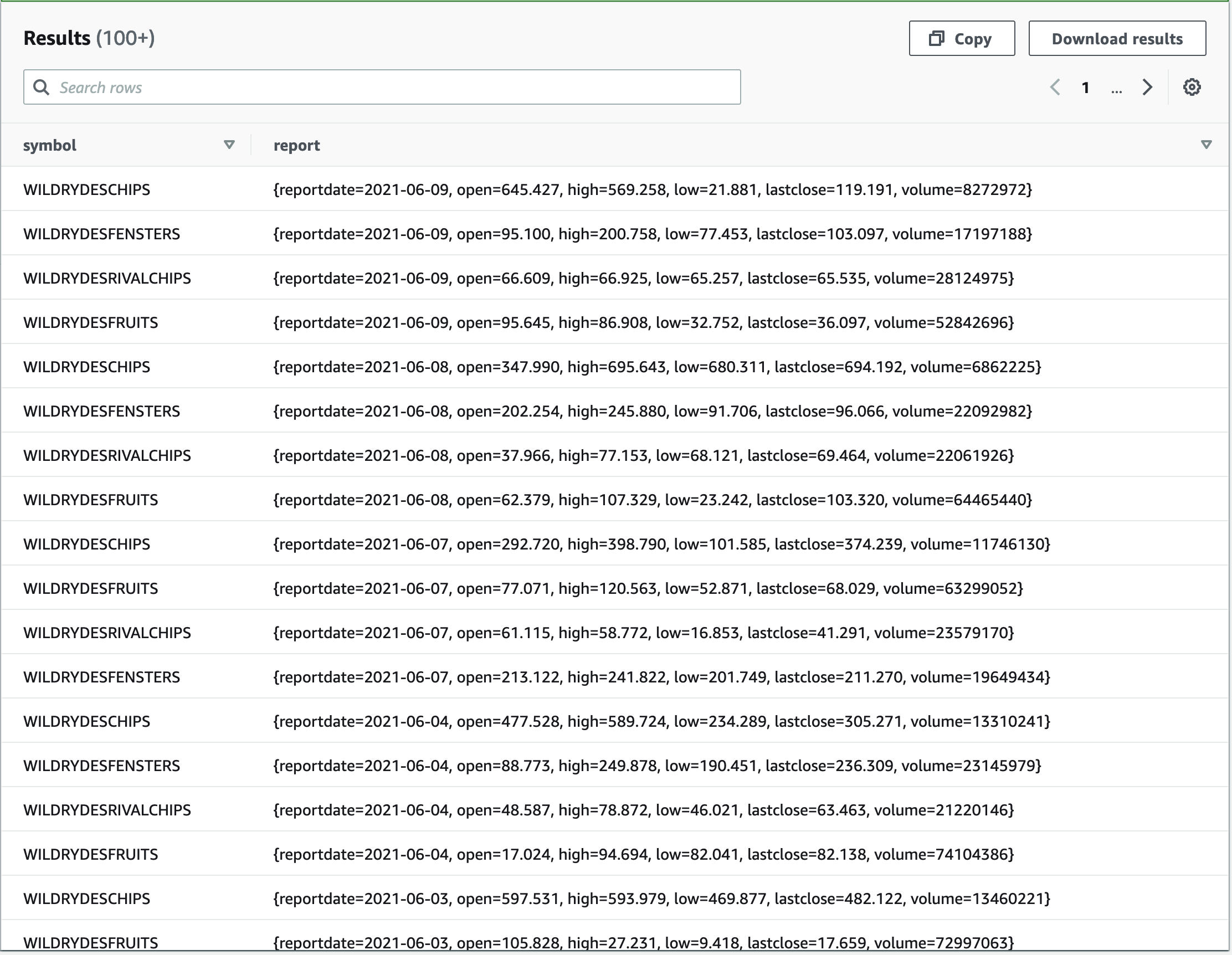
If you followed along with the simplified example, it should be easy now to see how we can apply this method to our financial reports:
We get the following results.
Bam! Now that was easy, wasn’t it?
With this as a basis, let’s select the data that we want to provide to our business users and turn the query into a view. The underlying data has still not been touched, is still formatted as JSON, and is still expressed using nested hierarchies. The new view makes all this transparent and provides a tabular view.
Let’s create the view:
Then we check our work:
We get the following results.
This is a good basis and acts as an interface for our business users.
The previous steps were based on the initial approach of mapping the JSON structures directly to columns. Let’s also explore the alternative path that we discussed before. What does this look like when we keep the data JSON formatted for longer, as we did in our alternative approach?
For variety, this approach also shows json_parse, which is used here to parse the whole JSON document and convert the list of financial reports and their contained key-value pairs into an ARRAY(MAP(VARCHAR, VARCHAR)). This array is used in the unnesting and its children eventually in the column projections. With element_at elements in the JSON, you can access the value by name. You can also see the use of WITH to define subqueries, helping to structure the SQL statement.
If you run the following query, it returns the same result as the earlier approach. You can also turn this query into a view.
Visualize the data
Let’s get back to our example. We created the financial_reports_view that acts as our interface to other business intelligence tools. In this post, we use it to provide data for visualization using QuickSight. QuickSight can directly access data through Athena. Its pay-per-session pricing enables you to put analytical insights into the hands of everyone in your organization.
Let’s set this up together. We first need to select our view to create a new data source in Athena, then we use this data source to populate the visualization.
We’re creating the visual that we shared at the beginning of this post. If you want just the data and you’re not interested in condensing data to a visual story, you can skip ahead to the post-conclusion section.
Create an Athena data source in QuickSight
Before we can use the data in QuickSight, we need to first grant access to the underlying S3 bucket. If you haven’t done so already for other analyses, see Accessing Data Sources for instructions. To create a dataset, complete the following steps (see Creating a Dataset Using Amazon Athena Data for more information):
- On the QuickSight console, choose Datasets.
- Choose New dataset.
- Choose Athena as the data source.
- For Data source name, enter a descriptive name.
- Choose Create data source.

- Choose the default database and our view
financial_reports_view. - Choose Select to confirm.
If you used multiple schemas in Athena, you could select them here as your database.

- In the next dialog box, you can choose to import the data into SPICE for quicker analytics or to directly query the data.

SPICE is the super-fast, parallel, in-memory calculation engine in QuickSight. For our example, you can go either way. Using SPICE results in the data being loaded from Athena only once, until it’s either manually refreshed or automatically refreshed (using a schedule). Using direct query means that all queries are run on Athena.
Our view now is a data source for QuickSight and we can turn to visualizing the data.
Create a visual in QuickSight
You can see the data fields on the left. Notice that reportdate is shown with a calendar symbol and lastclose as a number. QuickSight picks up the data types that we defined in Athena.
The sheet on the right is still empty.

Before we populate it with data, let’s choose Line chart from the available visual types.

To populate the graph, drag and drop the fields from the field list onto their respective destinations. In our case, we put reportdate onto the X axis well. We put our metric lastclose onto the Value well, so that it’s displayed on the y-axis. We put the symbol onto the Color well, which helps us tell the different stocks apart.

An initial version of our visualization is now shown on the canvas. Drag the handle at the lower-right corner to adjust the size to your liking. Also, choose the gear icon from the drop-down menu in the upper right corner. Doing this opens a dialog with more options to enhance the visualization.
Expand the Data labels section and choose Show data labels. Your changes are immediately reflected in the visualization.

You can also interact with the data directly. Given that QuickSight picked up on the reportdate being a DATE, it provides a date slider at the bottom of the visual. You can use this slider to adjust the time frame shown.
You can add further customizations. These can include changing the title of the visual or the axis, adjusting the size of the visual, and adding additional visualizations. Other possible customizations are adding data filters and capturing the combination of visuals into a dashboard. You might even turn the dashboard into a scheduled report that gets sent out once a day by email.
Further Considerations
More on using JSON
JSON features blend nicely into the existing SQL oriented functions in Athena, but aren’t ANSI SQL compatible. Also, the JSON file is expected to carry each record in a separate line.
In the documentation for the JSON SerDe libraries, you can find how to use the property ignore.malformed.json to indicate if malformed JSON records should be turned into nulls or an error. Further information about the two possible JSON SerDe implementations is linked in the documentation. If necessary, you can dig deeper and find out how to take explicit control of how column names are parsed, for example to avoid clashing with reserved keywords.
How to efficiently store data
During our experiments, we never touched the actual data. We only defined different ways to interpret the data. This approach works well for us here, because we’re only dealing with a small amount of data. If you want to use these concepts at scale, consider how to apply partitioning of data and possibly how to consolidate data into larger files.
Depending on the data, also consider whether storing it in a columnar fashion, using for example Apache Parquet, might be beneficial. You can find additional practical suggestions in Top 10 Performance Tuning Tips for Amazon Athena.
All these options don’t replace what you learned in this post, but benefit from your being able to compare and contrast JSON-formatted data and nested data. They can be used in a complementary fashion.
For a real-world scenario showing how to store and query data efficiently, see Analyze your Amazon CloudFront access logs at scale.
Conclusion
We have seen how to use JSON-formatted data that is stored in Amazon S3. We contrasted two approaches to map the JSON-formatted data to data structures in Athena:
- Mapping the JSON structures at table creation time to columns.
- Leaving the JSON structures untouched and instead mapping the contents as a whole to a string, so that the JSON contents remains intact. The JSON contents can later be interpreted and the structures at query creation time mapped to columns.
The approaches are not mutually exclusive, but can be used in parallel for the same underlying data.
Furthermore, JSON data can be hierarchical, which must be unnested and cross-joined to provide the data in a flattened, tabular fashion.
For our example, we provided the data in a tabular fashion and created a view that encapsulates the transformations, hiding the complexity from its users. We used the view as an interface to QuickSight. QuickSight directly accesses the Athena view and visualizes the data.
About the Authors
 Mariano Kamp is a principal solutions architect with Amazon Web Services. He works with financial services customers in Germany and has more than 25 years of industry experience covering a wide range of technologies. His area of depth is Analytics. In his spare time, Mariano enjoys hiking with his wife.
 John Mousa is a Senior Solutions Architect at AWS. He helps power and utilities and healthcare and life sciences customers as part of the regulated industries team in Germany. John has interest in the areas of service integration, microservices architectures, as well as analytics and data lakes. Outside of work, he loves to spend time with his family and play video games.
Audit History
Last reviewed and updated in April 2024 by Priyanka Chaudhary | Sr. Solutions Architect