AWS Big Data Blog
Use unsupervised training with K-means clustering in Amazon Redshift ML
June 2023: This post was reviewed and updated for accuracy.
Amazon Redshift is a fast, petabyte-scale cloud data warehouse delivering the best price–performance. Tens of thousands of customers use Amazon Redshift to process exabytes of data every day to power their analytics workloads. Data analysts and database developers want to use this data to train machine learning (ML) models, which can then be used to generate insights for use cases such as forecasting revenue, predicting customer churn, and detecting anomalies.
Amazon Redshift ML makes it easy for SQL users to create, train, and deploy ML models using familiar SQL commands. In previous posts, we covered how Amazon Redshift supports supervised learning that includes regression, binary classification, and multiclass classification, as well as training models using XGBoost and providing advanced options such as preprocessors, problem type, and hyperparameters.
In this post, we use Redshift ML to perform unsupervised learning on unlabeled training data using the K-means algorithm. This algorithm solves clustering problems where you want to discover groupings in the data. Unlabeled data is grouped and partitioned based on their similarities and differences. By grouping, the K-means algorithm iteratively determines the best centroids and assigns each member to the closest centroid. Data points nearest the same centroid belong to the same group. Members of a group are as similar as possible to other members in the same group, and as different as possible from members of other groups. To learn more about K-means clustering, see K-means clustering with Amazon SageMaker.
Solution overview
The following are some use cases for K-means:
- Ecommerce and retail – Segment your customers by purchase history, stores they visited, or clickstream activity.
- Healthcare – Group similar images for image detection. For example, you can detect patterns for diseases or successful treatment scenarios.
- Finance – Detect fraud by detecting anomalies in the dataset. For example, you can detect credit card fraud by abnormal purchase patterns.
- Technology – Build a network intrusion detection system that aims to identify attacks or malicious activity.
- Meteorology – Detect anomalies in sensor data collection such as storm forecasting.
In our example, we use K-means on the Global Database of Events, Language, and Tone (GDELT) dataset, which monitors world news across the world, and the data is stored for every second of every day. This information is freely available as part of the Registry of Open Data on AWS.
The data is stored as multiple files on Amazon Simple Storage Service (Amazon S3), with two different formats: historical, which covers the years 1979–2013, and daily updates, which cover the years 2013 and later. For this example, we use the historical format and bring in 1979 data.
For our use case, we use a subset of the data’s attributes:
- EventCode – The raw CAMEO action code describing the action that
Actor1performed uponActor2. - NumArticles – The total number of source documents containing one or more mentions of this event. You can use this to assess the importance of an event. The more discussion of that event, the more likely it is to be significant.
- AvgTone – The average tone of all documents containing one or more mentions of this event. The score ranges from -100 (extremely negative) to +100 (extremely positive). Common values range between -10 and +10, with 0 indicating neutral.
- Actor1Geo_Lat – The centroid latitude of the
Actor1landmark for mapping. - Actor1Geo_Long – The centroid longitude of the
Actor1landmark for mapping. - Actor2Geo_Lat – The centroid latitude of the
Actor2landmark for mapping. - Actor2Geo_Long – The centroid longitude of the
Actor2landmark for mapping.
Each row corresponds to an event at a specific location. For example, rows 53-57 in the file 1979.csv which we will use below, seem to all refer to interactions between FRA and AFR, dealing with consultation and diplomatic relations with a mostly positive tone. It is hard, if not impossible for us to make sense of such data at scale. Clusters of events, either with a similar tone, occurring in similar locations or between similar actors, are useful in visualizing and interpreting the data. Clustering can also reveal non-obvious structures such as potential common causes for different events, or the propagation of a root event across the globe, or the change in tone toward a common event over time. However, we do not know what makes two events similar – is it the location, the two actors, the tone, the time or some combination of these? Clustering algorithms can learn from data and determine 1) what makes different datapoints similar, 2) which datapoints are related to which other datapoints and 3) what are the common characteristics of these related datapoints.
Prerequisites
To get started, we need an Amazon Redshift cluster with version 1.0.33433 or higher and an AWS Identity and Access Management (IAM) role attached that provides access to Amazon SageMaker and permissions to an S3 bucket.
For an introduction to Redshift ML and instructions on setting it up, see Create, train, and deploy machine learning models in Amazon Redshift using SQL with Amazon Redshift ML.
To create a simple cluster, complete the following steps:
- On the Amazon Redshift console, choose Clusters in the navigation pane.
- Choose Create cluster.
- Provide the configuration parameters such as cluster name, user name, and password.
- For Associated IAM roles, on the menu Manage IAM roles, choose Create IAM role.
If you have an existing role with the required parameters, you can choose Associate IAM roles.
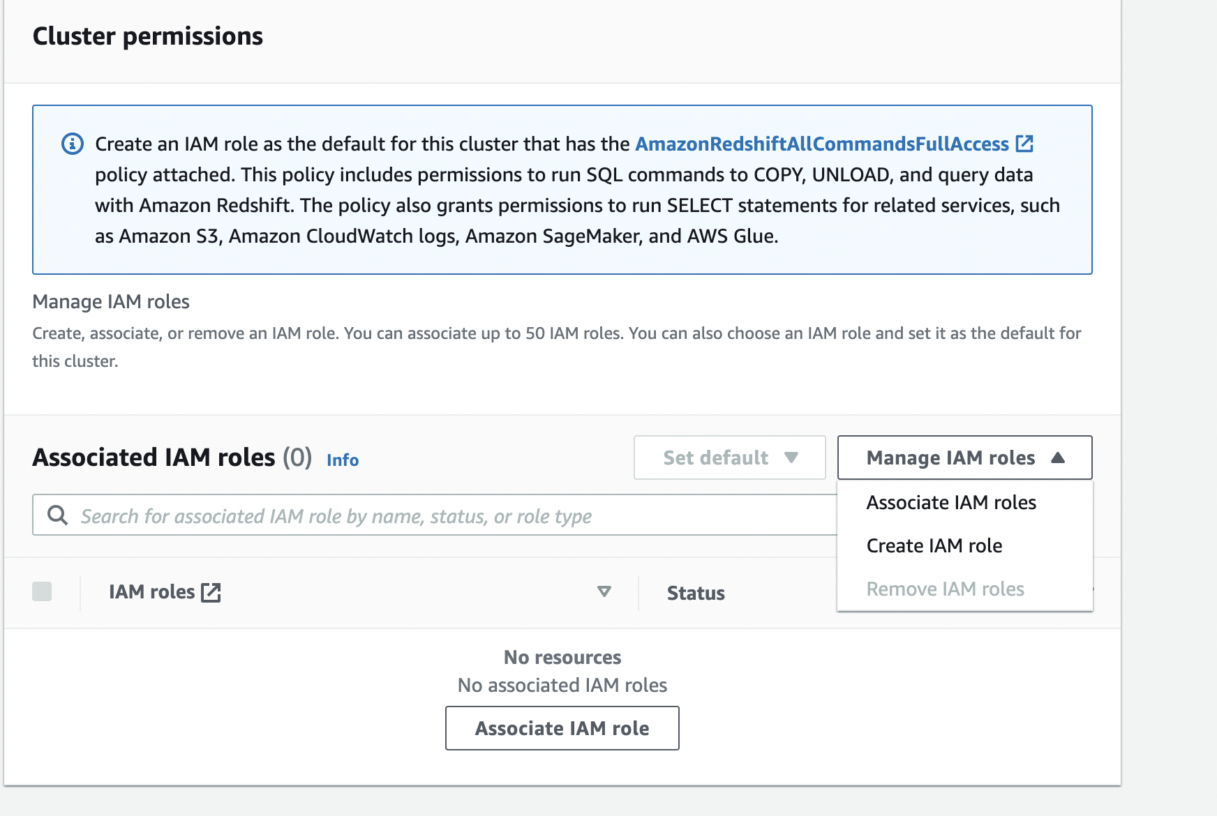
- Select Specific S3 buckets and choose a bucket for storing the artifacts generated by Redshift ML.
- Choose Create IAM role as default.

A default IAM role is created for you and automatically associated with the cluster.
- Choose Create cluster.

Prepare the data
Load the GDELT data into Amazon Redshift using the following SQL. You can use the Amazon Redshift Query Editor v2 or your favorite SQL tool to run these commands.
To create the table, use the following commands:
To load data into the table, use the following command:
Create a model in Redshift ML
When using the K-means algorithm, you must specify an input K that specifies the number of clusters to find in the data. The output of this algorithm is a set of K centroids, one for each cluster. Each data point belongs to one of the K clusters that is closest to it. Each cluster is described by its centroid, which can be thought of as a multi-dimensional representation of the cluster. The K-means algorithm compares the distances between centroids and data points to learn how different the clusters are from each other. A larger distance generally indicates a greater difference between the clusters.
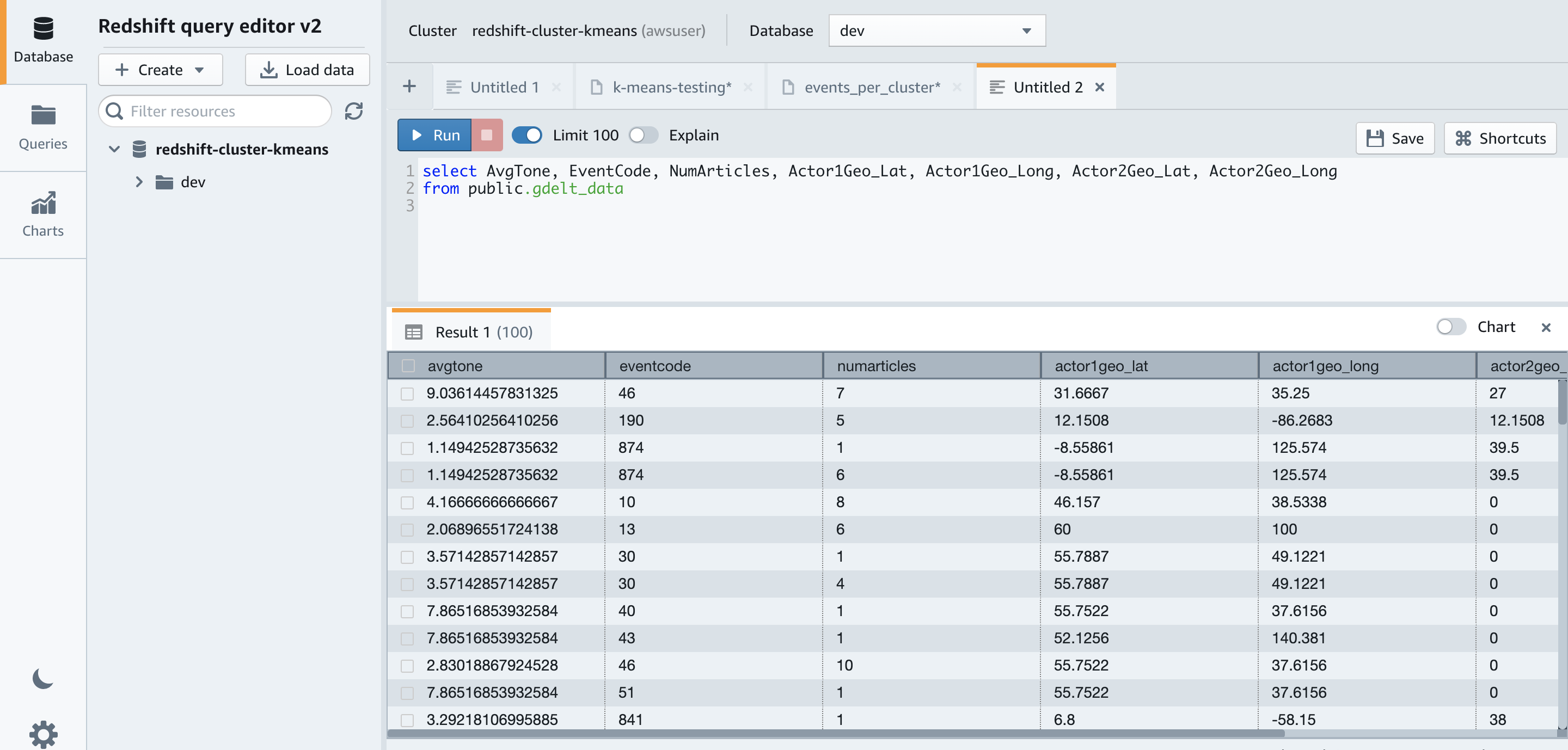
Before we create the model, let’s examine the training data by running the following SQL code in Amazon Redshift Query Editor v2:
The following screenshot shows our results.
We create a model with seven clusters from this data (see the following code). You can experiment by changing the K value and creating different models. The SageMaker K-means algorithm can obtain a good clustering with only a single pass over the data with very fast runtimes.
For more information about model training, see Machine learning overview. For a list of other hyper-parameters K-means supports, see K-means Hyperparameters, for the full syntax of CREATE MODEL see our documentation.
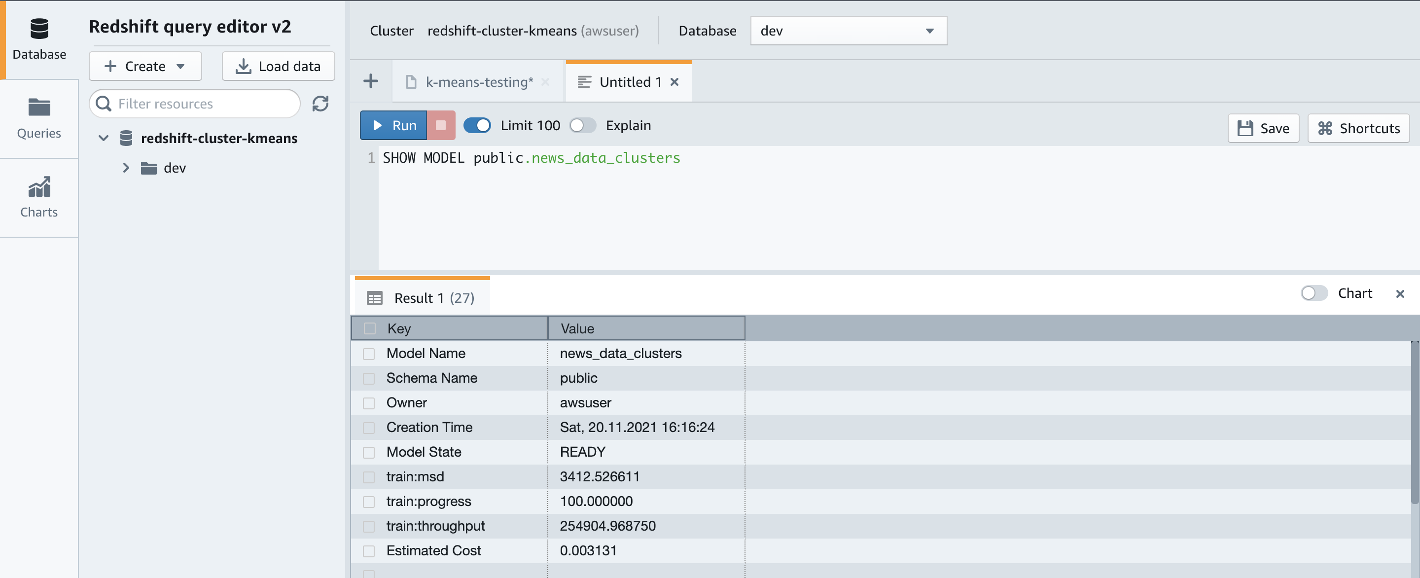
You can use the SHOW MODEL command to view the status of the model:
The results show that our model is in the READY state.
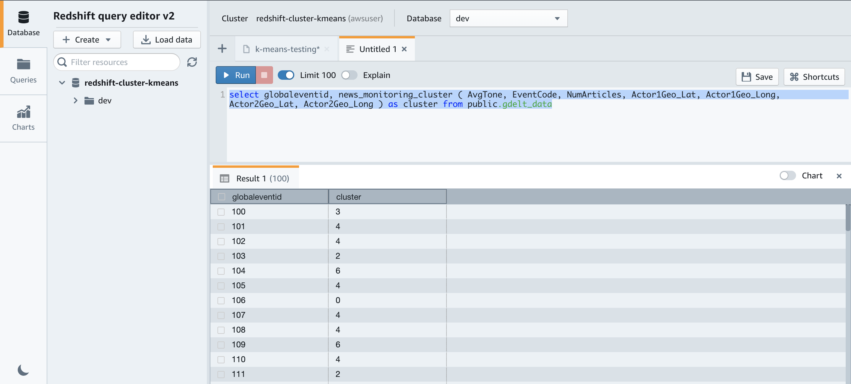
We can now run the query to identify the clusters. The following query shows the cluster associated with each GlobelEventId:
We get the following results.
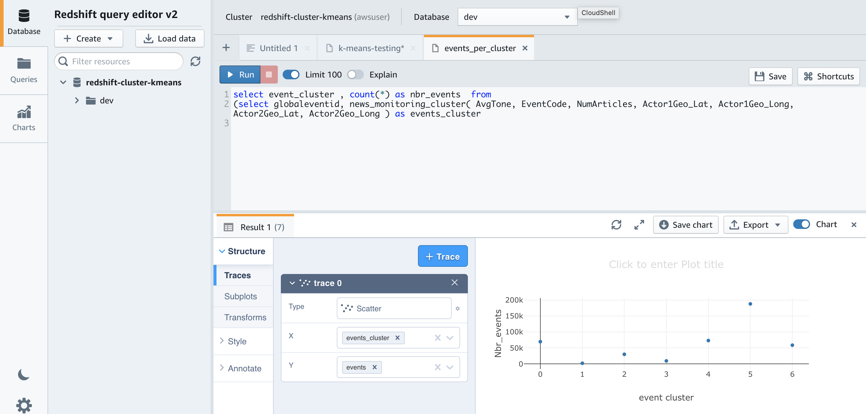
Now let’s run a query to check the distribution of data across our clusters to see if seven is the appropriate cluster size for this dataset:
The results show that very few events are assigned to clusters 1 and 3.
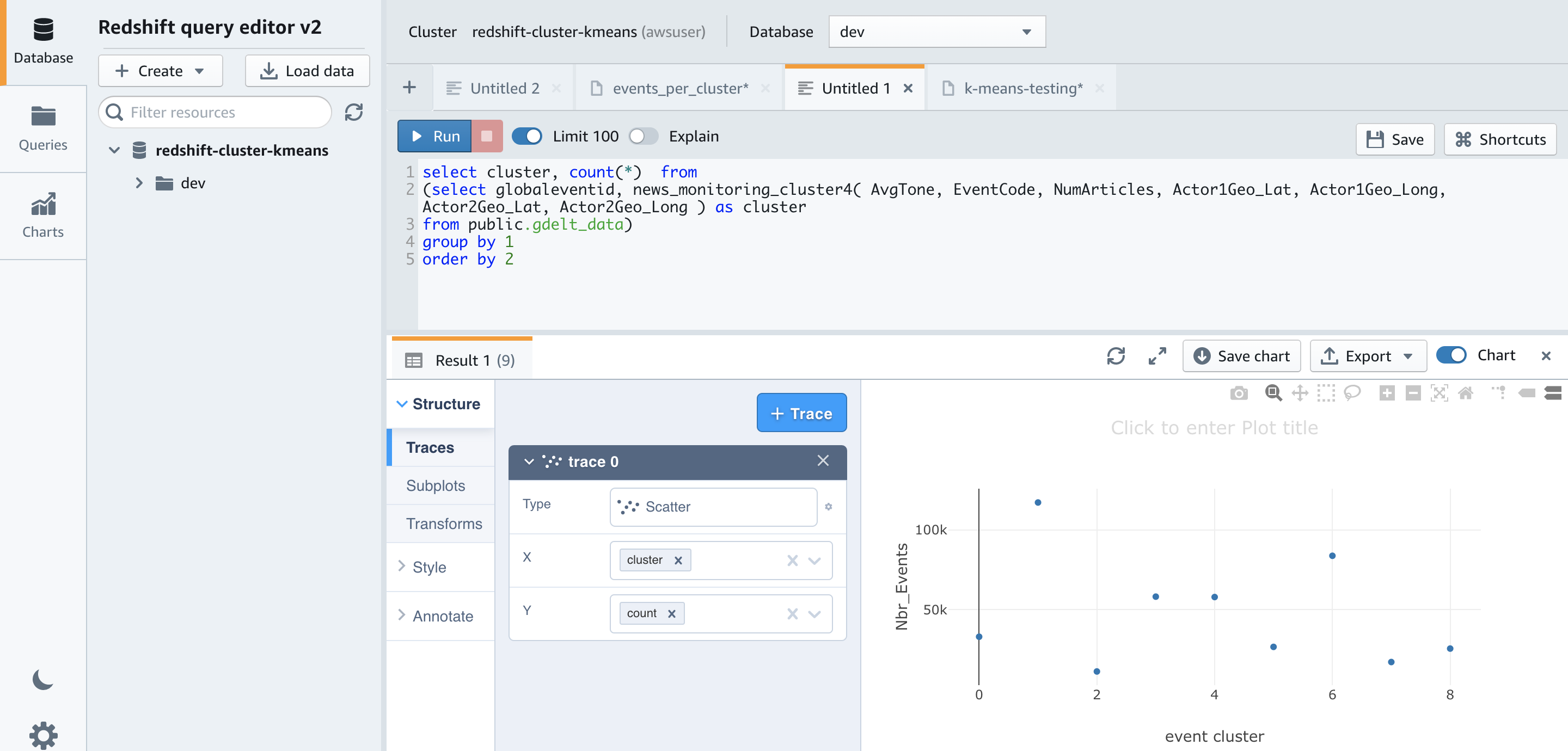
Let’s try running the above query again after re-creating the model with nine clusters by changing the K value to 9.
Using nine clusters helps smooth out the cluster sizes. The smallest is now approximately 11,000 and the largest is approximately 117,000, compared to 188,000 when using seven clusters.
Now, let’s run the following query to determine the centers of the clusters based on number of articles by event code:
Let’s run the following query to get more insights into the datapoints assigned to one of the clusters:
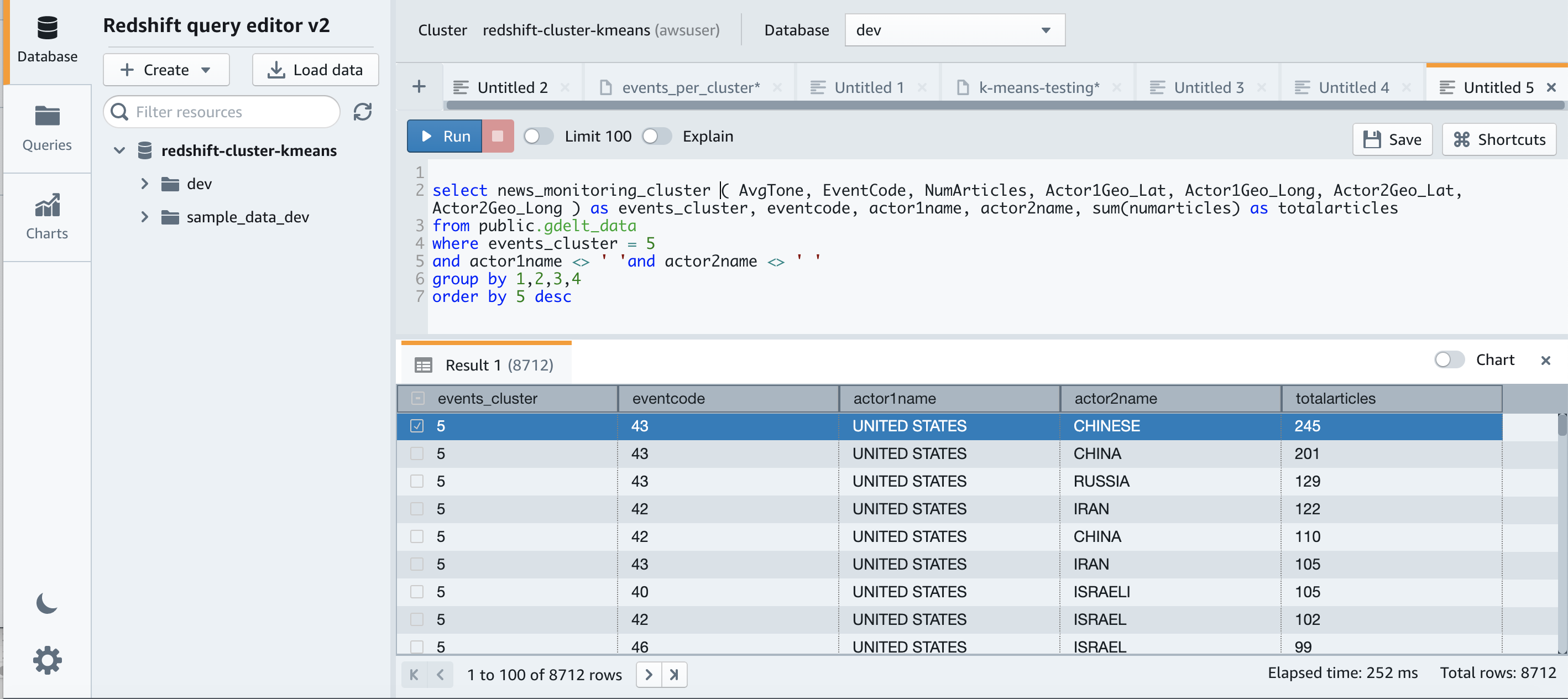
Observing the datapoints assigned to the clusters, we see clusters of events corresponding to interactions between US and China – probably due to the establishment of diplomatic relations, between US and RUS – probably corresponding to the SALT II Treaty and those involving Iran– probably corresponding to the Iranian Revolution. Thus, clustering can help us make sense of the data, and show us the way as we continue to explore and use it.
Conclusion
Redshift ML makes it easy for users of all skill levels to use ML technology. With no prior ML knowledge, you can use Redshift ML to gain business insights for your data. You can take advantage of ML approaches such as supervised and unsupervised learning to classify your labeled and unlabeled data, respectively. In this post, we walked you through how to perform unsupervised learning with Redshift ML by creating an ML model that uses the K-means algorithm to discover grouping in your data.
For more information about building different models, see Amazon Redshift ML.
About the Authors
 Phil Bates is a Senior Analytics Specialist Solutions Architect at AWS with over 25 years of data warehouse experience.
 Debu Panda, a Principal Product Manager at AWS, is an industry leader in analytics, application platform, and database technologies, and has more than 25 years of experience in the IT world. Debu has published numerous articles on analytics, enterprise Java, and databases and has presented at multiple conferences such as re:Invent, Oracle Open World, and Java One. He is lead author of the EJB 3 in Action (Manning Publications 2007, 2014) and Middleware Management (Packt).
 Akash Gheewala is a Solutions Architect at AWS. He helps global enterprises across the high tech industry in their journey to the cloud. He does this through his passion for accelerating digital transformation for customers and building highly scalable and cost-effective solutions in the cloud. Akash also enjoys mental models, creating content and vagabonding about the world.
 Murali Narayanaswamy is a principal machine learning scientist in AWS. He received his PhD from Carnegie Mellon University and works at the intersection of ML, AI, optimization, learning and inference to combat uncertainty in real-world applications including personalization, forecasting, supply chains and large scale systems.