AWS Big Data Blog
Get started with Amazon OpenSearch Service: T-shirt-size your domain
Welcome to this introductory series on Amazon OpenSearch Service. In this and future blog posts, we provide the basic information that you need to get started with Amazon OpenSearch Service.
Introduction
When you’re spinning up your first Amazon OpenSearch Service domain, you need to configure the instance types and count, decide whether to use dedicated masters, enable zone awareness, and configure storage. In this series, I’ve discussed using storage as a guideline for determining instance count, but I haven’t dug in on any other parameters. In this post, I offer some recommendations based on T-shirt sizing for log analytics workloads.
Log analytics and streaming workload characteristics
When you use Amazon OpenSearch Service for your streaming workloads, you send data from one or more sources into Amazon OpenSearch Service. Amazon OpenSearch Service stores your data (or more properly, an index of your data) in an index or indexes that you define. You further define time slicing and a retention period for the data to manage its lifecycle in your domain.
In the following figure, you have one data source producing a stream of data.
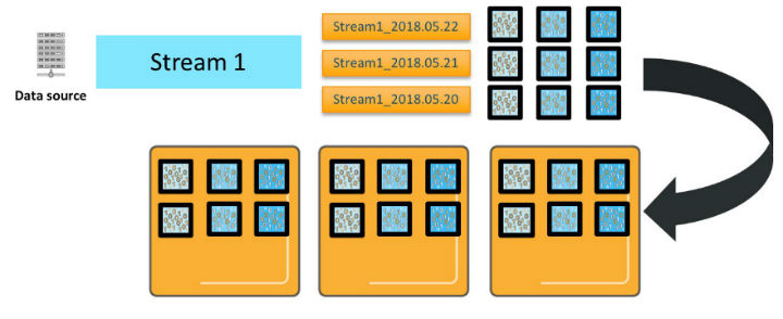
As you send that stream of data to Amazon OpenSearch Service, you create an index per day named Stream1_2018.05.21, Stream1_2018.05.22, and so on. We’ll call Stream1_ an index pattern. The diagram shows three primary shards for each of these indexes. The shards are deployed on three Amazon OpenSearch Service data instances, along with one replica for each of the primaries. (For simplicity, the diagram doesn’t show it, but the shards are deployed so that the primary and replica are on different instances.)
When Amazon OpenSearch Service processes an update, that update is sent to all of the primaries and replicas that are receiving new or updated documents.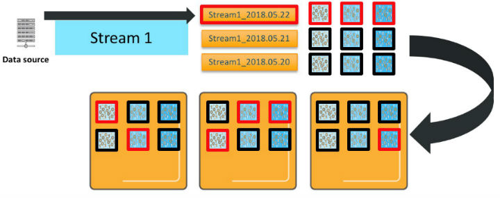
There are several important characteristics of how Amazon OpenSearch Service processes your updates. First, each index pattern deploys the number of primaries * number of replicas * number of days of retention total shards. Second, even though there are three indexes in this index pattern, time slicing means that new documents go to only one of these indexes—the active index for that index pattern. Third, assuming that you are sending _bulk data and it’s randomly distributed, every shard for that index receives and writes an update. So, for this index pattern, you need six vCPUs to process a single _bulk request.
Similarly, Amazon OpenSearch Service distributes queries across the shards for the indexes involved. If you query this index pattern across all three days, you will engage 18 shards, and need 18 vCPUs to process the request.
The picture gets even more complicated when you add in more data streams and index patterns. For each additional data stream/index pattern, you deploy shards for each of the daily indexes and use vCPUs to process requests in proportion to the shards deployed, as shown in the preceding diagram. When you make concurrent requests to more than one index, each shard for all of the indexes involved must process those requests.
Cluster capacity
As the number of index patterns and concurrent requests increases, you can quickly overwhelm the cluster’s resources. Amazon OpenSearch Service includes internal queues that buffer requests and mitigate this concurrency demand. You can see these queues and monitor their depth by using the _cat/thread_pool API.
Another complicating dimension is that the time to process your updates and queries depends on the contents of the updates and queries. As requests come in, the queues are filling at the rate you are sending them. And they are draining at a rate that is governed by the vCPUs that are available, the time they take on each request, and the processing time for that request. You can interleave more requests if those requests clear in a millisecond than if they clear in a second. A full conversation on this topic is out of scope for this post. You can use the _nodes/stats OpenSearch API to monitor average load on your CPUs.
If you see the queue depths increasing, you are moving into a “warning” area, where the cluster is handling load. But if you continue, you can start to exceed the available queues and need to scale to add more CPUs. If you start to see load increasing, which is correlated with queue depth increasing, you are also in a “warning” area and should consider scaling.
Recommendations
The following table recommends instances based on the amount of source data, the storage needed, and the active and total shards. As with all sizing recommendations, these guidelines represent a starting point. Try them out, monitor your Amazon OpenSearch Service domain, and adjust as needed.
| T-shirt size |
Data (per day) |
Storage needed | Active shards (maximum) |
Total shards (maximum) |
Instances |
|---|---|---|---|---|---|
| XSmall | 10 GB | 177 GB | 4 @ 50 GB |
300 | 2x M4/R4.large data 3x m3.medium masters |
| Small | 100 GB | 1.7 TB | 8 @ 50 GB |
600 | 4x M4/R4.xlarge data 3x m3.medium masters |
| Medium | 500 GB | 8.5 TB | 30 @ 50 GB |
3000 | 6x I3.2xlarge data 3x C4.large masters |
| Large | 1 TB | 17.7 TB | 60 @ 50 GB |
3000 | 6x I3.4xlarge data 3x C4.large masters |
| XLarge | 10 TB | 177.1 TB | 600 @ 50 GB |
5,000 | 30x I3.8xlarge data 3x C4.2xlarge masters |
| Huge | 80 TB | 1.288 PB | 3400 @ 50 GB |
25,000 | 85x I3.16xlarge data 3x C4.4xlarge masters |
NOTE: This table presents guidelines that are based on many assumptions. Your workload will differ, and so your actual needs will differ from these recommendations. Please make sure to deploy, monitor, and adjust!
At the low end, an extra-small use case encompasses 10 GB or less of data per day from a single data stream to a single index pattern. A small use case falls between 10 and 100 GB per day of data, a medium use case between 100 and 500 GB of data, and so on. At the huge end, Amazon OpenSearch Service supports up to 80 TB of data per day across one or many index patterns, for a total of more than a petabyte of stored data. For the extra-large and huge workloads, you need to request a limit raise beyond the default 20 data instances per domain.
To figure out the storage needed, I multiplied the data per day by an assumed source:index ratio of 1.1, doubled for a replica, and multiplied by 7, assuming a 7-day retention period.
Storage needed = Source bytes * 1.1 * 2 * 7 * 1.15
(Note that this recommendation includes an additional 15% storage for overhead, beyond our prior guidance to prevent hitting OpenSearch’s cluster.routing.allocation.disk.watermark.low.)
To account for CPU needs, I added a column with targets for the maximum number of active shards and a column with a maximum number of shards total. Although your throughput and latencies will vary widely based on your workload, you should use the values in the Active shards (maximum) column as an initial scale point. The values in that column are driven by the number of vCPUs that are deployed across the instances that are recommended. At the lower end, the ratio of active shards to CPUs is 1:1. At a larger scale, I’ve recommended fewer shards per instance to allow for more and heavier cluster tasks.
When you are planning for scale, you can map the number of index patterns onto the maximum active shards and scale accordingly. If you run a single index pattern, then the number of active shards for processing updates is the number of primaries plus the number of replicas. If you run two or more index patterns, it is the sum of the active shards across the active indexes.
The Active shards column also includes a recommendation for shard sizing. You control shard sizing by setting the count of primary shards for your index, given the size of the index on disk. See the post How Many Shards Do I Need? for details. We agree with Elastic’s recommendations on a maximum shard size of 50 GB.
The Total shards column gives you a guideline around the sum of all of the primary and replica shards in all indexes stored in the cluster, including active and older indexes. Use it to plan for your retention time and your overall storage strategy. The values in the Total shards column are driven by the amount of underlying RAM that is allocated to your Java virtual machine (JVM). Following Elastic’s guidelines, we recommend a maximum of 25 shards per GB of RAM allocated to the JVM.
The final column recommends instance counts and instance types for data and master instances in your Amazon OpenSearch Service domain. In all but the smallest use cases, we recommend the I3 instances. At $0.39 per GB hour of storage (us-east-1), it’s hard to beat these instances on cost. With their NVMe SSDs, disk and network bandwidth, RAM size, and CPU count, it’s also hard to beat these instances on performance. The exception is at the low end, where you can use smaller EBS volumes and optimize your storage needs to reduce cost.
Conclusion
Use the guidelines in this post as a starting point. Your workload will behave in its own unique way and will scale individually. Always monitor and scale appropriately. At the same time, you can use the techniques I’ve described in building these recommendations to interpolate and set some expectations to get you started on the right foot.
About the Author
 Jon Handler (@_searchgeek) is an AWS solutions architect specializing in search technologies. He works with our customers to provide guidance and technical assistance on database projects, helping them improve the value of their solutions when using AWS.