AWS Machine Learning Blog
Deploying custom models built with Gluon and Apache MXNet on Amazon SageMaker
When you build models with the Apache MXNet deep learning framework, you can take advantage of the expansive model zoo provided by GluonCV to quickly train state-of-the-art computer vision algorithms for image and video processing. A typical development environment for training consists of a Jupyter notebook hosted on a compute instance configured by the operating data scientist. To make sure this environment is replicated during use in production, the environment is wrapped inside a Docker container, which is launched and scaled according to the expected load. Hosting the deep learning model is a challenge that generally involves knowledge of server hosting, cluster management, web API protocols, and network security.
In this post, we demonstrate how Amazon SageMaker supports these libraries and how their integration simplifies the deployment of complex algorithms without having to build expertise in web app infrastructure. Whether inference constraints require real-time predictions with low latency, or irregularly-timed batch jobs with a large number of samples, optimal hosting solutions are available and easy to build.
With Amazon SageMaker, most of the undifferentiated heavy lifting is already done. There is no need to build out a container image from scratch or set up a REST API. Instead, you only need to specify various model functions to processes inference data in a manner consistent to the training pipeline. You can follow this post with an end-to-end example, in which we train an object detection model using open-source Apache tools.
Creating a notebook instance
You can run the example code we provide in this post. It’s recommended to run the code inside an Amazon SageMaker instance type of ml.p3.2xlarge or larger to accelerate training time. To create a notebook instance, complete the following steps:
- On the Amazon SageMaker console, choose Notebook instances.
- Choose Create notebook instance.
- Enter the name of your notebook instance, such as
mxnet-gluon-deployment. - Set the instance type to p3.2xlarge.
- Choose Additional configuration.
- Set the volume size to 20 GB.
- Choose Create notebook instance.
- When the instance is ready, choose Open in JupyterLab.
- From the launcher, you can open a terminal and run the provided code.
Generating the model
For this use case, you build an object detection model using a pretrained Faster R-CNN architecture from the GluonCV model zoo on the Pascal VOC dataset. The first step is to obtain the data, which you can do by running the data preparation script pascal_voc.py for use with GluonCV. The script downloads 8.4 GB of annotated images to ~/.mxnet/datasets/voc/. With the dataset in place, run the training script train_faster_rcnn.py from this GluonCV example.
Model parameters are saved after each epoch, with the best performing model indicated by the suffix _best.params.
Preparing the inference container image
To make sure that the compute environment for the inference instance is set according to our needs, run the model within a Docker container that specifies the required configuration. Containers provide a portable, efficient, standalone package of software for flexible deployment. In most cases, using the default MXNet inference container image in Amazon SageMaker is sufficient for hosting Apache MXNet models. However, we built a computer vision model using GluonCV, which isn’t included in the default image. You can now modify the MXNet inference container image to include GluonCV, which you use for deployment.
Our instance requires Docker for the following steps, which is included in Amazon SageMaker instances. First clone the Amazon SageMaker MXNet serving container GitHub repository:
Included in the repo is a Dockerfile that serves our configuration with MXNet 1.6.0, GluonCV 0.6.0, and Python 3.6.8. You can verify the software versions in ./docker/1.6.0/py3/Dockerfile.gpu:
There is no need to edit this file for this post, but you can add additional packages to the preceding code as needed.
Now you build the container image. Before executing the docker build command, copy the necessary artifacts to the ./docker/1.6.0/py3 directory. In the following example code, we use gluoncv-mxnet-serving:1.6.0-gpu-py3 as the name and the tag. Note the . at the end of the last command:
To test the container was built successfully, you can run the container locally. In the following code, replace <docker image id> and <container id> with the output from the commands docker images and docker ps:
In a separate terminal, access the shell of the running container:
To escape the terminals and tear down the resources, enter exit in the shell accessing the container and enter CTRL+C in the terminal running the container.
Now you’re ready to upload the new MXNet inference container image to Amazon Elastic Container Registry (Amazon ECR) so you can point to this container image when you deploy the model on Amazon SageMaker. For more information, see Pushing an image.
You first authenticate Docker to the Amazon ECR registry with get-login. Assuming the AWS Command Line Interface (AWC CLI) version is prior to 1.17.0, enter the following code to get the authenticated docker login command:
For instructions on using AWS CLI version 1.17.0 or higher, see Using an Authorization Token.
Copy the output of the command, then paste and execute it to authenticate your Docker installation into Amazon ECR. Replace with the appropriate Region. For example, to use the US East (N. Virginia) Region, replace with us-east-1.
Create a repository in Amazon ECR using the AWS CLI by running aws ecr create-repository. For this use case, use gluconcv for <repository name>:
Before pushing the local image to Amazon ECR, tag it with the name of the target repository. The image ID is retrieved with the docker images command and named with the docker tag command and the repository URI, which you can also retrieve on the Amazon ECR console. See the following code:
To push the image to the Amazon ECR repository so that it’s available for hosting on Amazon SageMaker endpoints, use the docker push command. You can confirm that the image is successfully pushed using the aws ecr list-images AWS CLI command:
Alternatively, you can verify the image exists in the repository by checking on the Amazon ECR console.
When deploying the model, use the image URI as the argument to image. You can run the code to set up the image programmatically from a Jupyter notebook:
Deploying the model
You can optimize compute resources according to inference requirements based on your use case. If you collect batches of data intermittently and don’t need predictions, you can run batch jobs over the data acquired by spinning up a compute instance when necessary, then process the mass of data, store the predictions, and tear down the instance.
Alternatively, you may require that calls for inference be answered immediately. In this case, spin up a compute instance for real-time inference at an endpoint that consumes data over an API call and returns the model output. You only pay for time when the compute instance is running. We provide details for both use cases in this section.
Prepare the model artifacts by compressing them into a tarball and uploading to Amazon S3, from which the deployed model is read. Because you’re using an architecture that already exists in the GluonCV model, you only need to upload the weights. The .params file from the previous step should ultimately live in s3://<bucket_name>/<prefix>/model.tar.gz. You execute deployment via the Amazon SageMaker SDK. See the following code:
The image ARN argument is the URI of the image you uploaded to the Amazon ECR repository in the preceding section. Make sure that the Region of the Amazon ECR repository and Amazon SageMaker model are the same. Most of the processing, inference, and configuration resides in the following entry_point.py script, which defines the model and the steps necessary to decode the payload so that the MXNet backend properly interprets the data:
entrypoint.py
After you import the supporting libraries for model inference and data processing, define the model in model_fn() by loading the Faster R-CNN architecture and the trained weights you uploaded to Amazon S3. The file name passed in the net.load_parameters() must match the name of the parameters file that you trained and uploaded to Amazon S3 earlier in the tarball. For this use case, the parameters are stored in faster_rcnn_resnet50_v1b_voc_best.params. To utilize the GPU, you must explicitly set the context as such when loading the parameters.
Instructions to run predictions over the model are written in transform_fn(). You can call inference from a living endpoint API or launch it on schedule for batch jobs. The corresponding data type sent to the model varies between these two options. When sent for a real-time prediction over the endpoint API, the transform function receives a string that you can load and interpret according to its underlying data type. Batch transform jobs, on the other hand, send the data directly as a serialized image, which you need to decode with MXNet utilities. You can handle both cases by checking the type of the data object.
The loaded data is normalized according to the default preprocessing steps that GluonCV implements, as enforced in the normalize() function in the entry point script. Lastly, the data is passed through the neural network for inference with the output formatted such that the return payload includes the predicted class ID, confidence of the bounding box, and bounding box attributes.
With all the setup in place, you’re now ready to deploy. See the following code:
Testing
With the deployed endpoint up and running, you can make a real-time inference with the returned object from the preceding step. After loading an image into a NumPy array, fire it off for inference:
To visualize the output, draw from the metadata included in the response. See the following code:
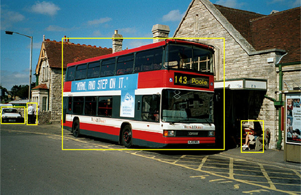
After 20 epochs of training, you can see bounding boxes that accurately identifying various objects in the model response. See the following screenshot.
The purpose of maintaining an endpoint API is to support a model to be available for real-time predictions. It’s unnecessary to pay for a running endpoint instance if inference jobs are scheduled in advance. For this use case, you send a list of images for prediction to a batch transform job, which spins up a compute instance to run the model and tears it down upon completion. You only pay for the runtime of the instance, which saves costs on downtime. Set up and launch a batch transform job by uploading images to Amazon S3 and defining the data and model paths, along with a few other settings, to a dictionary. See the following code:
You can verify the output of the batch transform job by comparing the output of the real-time inference, endpoint_response, to the output from the batch transform job, which was saved to s3://<bucket_name>/test/<batch_job_name>/2010_001453.jpg.out as specified in the S3OutputPath parameter.
Cleaning up
To finish up this walkthrough, tear down the endpoint instance and remove the Amazon SageMaker model. For more information about additional helper methods, see Using Estimators. Delete the Amazon ECR repository and its images through the Amazon ECR client. See the following code:
Conclusion
Although training models is a data scientist’s the primary objective, the deployment process is equally crucial. Amazon SageMaker offers efficient methods to put these algorithms into production. Built-in algorithms can accelerate the training process, but you may need custom modeling for your use case. When building a model with MXNet, you must specify the configuration and processing steps necessary to run it in production. For this post, we outlined the steps to load our model to Amazon SageMaker and run inference for real-time predictions and in batch jobs.
About the Authors
 Hussain Karimi is a data scientist at the Maching Learning Solutions Lab where he works with customers across various verticals to initate and build automated, algorithmic models that generate business value.
 Will Gleave is a Machine Learning Consultant with the NatSec team at AWS Professional Services. In his spare time, he enjoys reading, watching sports, and traveling.
 Muhyun Kim is a data scientist at Amazon Machine Learning Solutions Lab. He solves customer’s various business problems by applying machine learning and deep learning, and also helps them gets skilled.