AWS for M&E Blog
Optimizing computing performance with AWS Thinkbox Deadline – Part 1
AWS Thinkbox Deadline is a compute management solution often employed in the Media & Entertainment (M&E) and Architecture, Engineering and Construction (AEC) industries. It is used to control render farms with physical and virtual machines running both on-premises and on AWS.
Once Deadline is up and running, it is natural to look into how to get the best performance. The performance of the system can be measured in terms of speed (producing results faster), and in terms of cost (producing results cheaper). We would like to stay away from extremes like “Cheap but Slow” or “Fast but Expensive”, and find the right balance. Obviously, “Cheap and Fast” would be the desired outcome, and there are a lot of factors that can help us get closer to it.
In this three-part blog series, we will take a deep dive into the plethora of practical considerations related to maximizing the performance and keeping the cost of your Deadline-controlled computing resources in check, whether on-premises, on AWS, or in a hybrid environment.
A basic familiarity with AWS Thinkbox Deadline, 3D rendering workflows, and AWS EC2 offerings is assumed as a pre-requisite for the following discussion.
This blog is divided in three parts. In this first part, we will look at the hardware and software components of the render farm. In Part 2, we will discuss the Deadline features designed to maximize performance, and in part 3, the best ways to configure Deadline’s AWS Portal for fast and effective cloud rendering.
Measuring Performance
The factors influencing the performance like hardware, software, licenses, time schedules and budgets are tightly interconnected – tweaking one of them can have a significant impact on the others. While it is easy to answer the question “Which CPU or EC2 instance type is the fastest in absolute terms?”, it is much harder to answer “How do I finish my renders before the delivery deadline and within budget?”
We will need to gain a deeper understanding on how the performance is measured, how various factors like hardware and software configurations affect the performance, and how the price of resources influences our decisions.
To start, we will need performance data. Some of it, like the CPU type and clock frequency, memory amount, or EC2 instance price per hour, is readily available. We will have to collect the rest ourselves.
Using Benchmarks and Production Tests
Most render engines offer a standardized benchmark test – either implemented as a stand-alone utility, a special mode of the renderer, or a pre-packaged scene with assets to render. These benchmarks are typically based on one or more real-world scenes supplied by customers and beta testers, so they aren’t “synthetic” benchmarks. But they might not make use of all the features that your actual production scene calls for. For this reason, standard benchmarks are mainly useful for two purposes:
- Establishing the performance baseline of existing hardware – you can rank your hardware from slow to fast.
- Comparing existing on-premises hardware capabilities to EC2 instance type configurations – you can find the cloud instance types to match or exceed the performance of on-premises render nodes.
While you can make some educated guesses about how two different machine configurations would compare in performance in your own production scene based on their benchmark scores, it is a much better idea to use actual representative production scenes that push the relevant features of the software and hardware to make predictions about their real-world performance.
An important quality which not all benchmarks possess is consistency. It is generally recommended to run multiple benchmark tests on the same hardware and average the results to remove any deviations. However, most well-implemented benchmarks will invariably produce nearly the same values on the same type of hardware between runs. Unfortunately this is not true for all of them – at least one test that is popular on some technology websites for comparing hardware computing performance has shown inconsistent results between runs within the same session, most probably due to the influence of various CPU caches. So before you rely on the results of a benchmark, please be sure to run it several times in the same session and in multiple sessions to confirm its values are consistent!
A fairly consistent CPU benchmark (which also has a GPU component) is the V-Ray Benchmark based on Chaos Group’s V-Ray renderer. It also has a public repository of benchmark results, allowing you to measure your hardware performance against the rest of the world.
When this blog was originally published in December 2018, the build of the V-Ray Benchmark was based on V-Ray v3.5. It used bucket rendering for its CPU test and the results were expressed as the render time of the specific scene in minutes and seconds.

In 2019, Chaos Group released a new Benchmark based on V-Ray Next which runs progressive CPU rendering for exactly one minute, and returns a result expressed in thousands of samples per minute. For the GPU rendering benchmark, it returns the millions of paths traced in a minute.
PERFORMANCE VS. COST OPTIMIZATION
It is obvious that using larger EC2 instance types with many vCPUs would typically reduce the render time of a 3D image in absolute terms. Using 96 cores instead of 16 will definitely produce a faster rendering. However, while the cost per hour of the different instance sizes within an EC2 family like the Compute-optimized c5 or the General Purpose m5 grows linearly with the vCPU count, the rendering performance usually does not scale in a linear manner, especially with a very large number of vCPUs. So for example a c5.18xlarge with 72 vCPUs has an On-Demand cost that is exactly twice as much per hour as a c5.9xlarge with 36 vCPUs, but the performance measured by the V-Ray Benchmark is 44,383 ksamples vs 24,638 ksamples. The performance scaling factor from doubling the vCPU count is thus 1.8x and not the hoped for 2.0x.
Due to the above scaling behavior, it follows that selecting a smaller instance type, while rendering slower in absolute terms, can actually produce results at a lower cost per image! And since rendering an animation or even a single large image split into smaller segments can easily be done in parallel, launching many smaller instances can be more cost effective than running a few larger ones. The main concern would be making sure the scene fits in the available memory of the particular smaller instance, since the memory scales in lockstep with the vCPU count.
On the other hand, if a small instance takes hours to render an image that takes minutes on a larger instance, and your workflow would benefit from faster iterations, then paying a slightly higher price for faster feedback could be worth it. After all, the artists waiting for the render output are the most expensive resource in a company, and faster iterations can result in higher productivity and higher quality output for your client, possibly bringing more business your way – something that is hard to measure, but is important to consider.
Also, while rendering tests show that computing an image sequence on many smaller instances can be faster than rendering on a single multi-core computing unit due to better CPU utilization, if the renderer in question is licensed per-node, it might be more cost-effective to use larger instances to reduce the number of licenses required. Again, a fine balancing act of performance vs. cost is required, and there is no one-size-fits-all solution.
Measuring The Cost Performance
With the old V-Ray 3.5-based benchmark, we took the render time produced by the benchmark and divided it by a full hour to compute the theoretical number of images that could be rendered within an hour (ignoring any overhead of loading assets and preparing the rendering). Dividing the cost per hour of an instance type by this number gave us a “Cost Per Image” value for that machine.
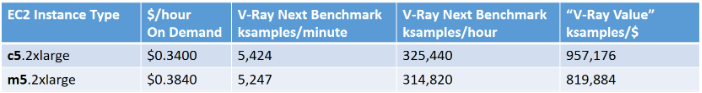
With the new V-Ray Next Benchmark, the render time is always constant, but the number of samples rendered is variable, so the quality of the produced image varies. If an instance produces twice as many samples in the same time, it will obviously achieve a particular quality twice as fast. For the cost calculation, instead of calculating a “Cost Per Image”, we can calculate a “V-Ray Value” expressing how many samples a dollar can buy. The calculation involves multiplying the benchmark result by 60 to turn the per-minute value to per-hour, and then dividing by the hourly price of the instance. We can then use the V-Ray Values which are calculated using the On-Demand, and especially the current regional EC2 Spot prices, to compare the cost performance of different instances.
In the example below, we can clearly see that the Compute Optimized c5.2xlarge instance type offers a higher value per dollar than a comparable General Purpose m5.2xlarge instance. This is mainly because the latter has twice the memory and thus costs a bit more, while delivering comparable benchmark scores.
Note that all examples in this blog are based on instance prices in the us-west-2 (Oregon) AWS Region. Your cost may vary depending on your Region.
Optimizing Resource Utilization
Picking the right software for the job
It might appear obvious, but selecting the right software tool is a very important consideration when optimizing a rendering pipeline. Every software tool exists for some good reason – either ease of use, speed, a good balance of both, a special feature no other tool offers, and so on. For that reason, deciding on the right tool for the job is not simple, and using the same tool on every job due to familiarity can be the wrong way to go.
Consider these questions
- Does the 3D tool or renderer offer any features that would make the particular job compute faster? For example, some renderers produce clean Global Illumination results more effectively, others excel in volumetric rendering, particle rendering, or fast sub-pixel displacement to produce higher quality images in less time.
- What is the licensing model and cost per hour for the tool and is there a cheaper alternative that produces comparable results?
- Does the renderer support GPU rendering? If yes, does the GPU implementation support all required features?
Picking the right hardware size
On-premises render farms often consist of many generations of hardware with different specifications, including
- CPU model, core count and frequency
- Chip maker (Intel, AMD)
- Micro-architecture (e.g. Ivy Bridge, Haswell, Broadwell, Skylake etc.)
- RAM amount
- GPU model, GPU count, CUDA cores, per-GPU memory
- Local disk drives
- Network adapter
Similarly, cloud instances, albeit running virtual machines on top of the hardware, generally offer either a pre-set number of instance types and sizes, or allow dynamic configuration of some of these components.
When selecting EC2 instances for CPU-based rendering, the Compute Optimized (C), General Purpose (M) and Memory Optimized (R) instance types should be on top of your list. Selecting from the more specialized categories like Accelerated Computing (P and G), Storage Optimized (H, I and D), or sub-categories of the Memory Optimized like X is not advisable – you would be paying for resources you don’t use. For GPU rendering, or hybrid CPU and GPU rendering, the P and G Accelerated Computing instances are of course not only fair game, but a requirement.
Like the machines of on-premises render farms, EC2 instances come not only in different sizes and configurations, but also in different generations. For example, at the time of this writing the current EC2 Compute, General Purpose, and Memory-Optimized instance types are at their 5th generation – C5, M5, and R5, respectively. Older generations such as C4 and C3 are still available, but just as one would expect, each newer generation scores higher in the performance benchmarks. What might be surprising though is that the newer generations of instances are also cheaper in both absolute and relative terms – their On-Demand price per hour goes down while the performance goes up! They should be your first choice when picking a list of render node candidates.
For example, the m3.2xlarge instance running Linux costs $0.532, the m4.2xlarge costs $0.4, and the m5.2xlarge is only $0.384, while their respective V-Ray Next CPU benchmarks go from 2,502 through 4,065 to 5,424 ksamples. In other words, the latest generation is more than 2x faster than the 3rd generation, while also being $0.148 cheaper. The combination of price and performance is especially obvious when looking at the ”V-Ray Value” of these instance types:

These differences are caused not only by improvements in the CPU and chipset designs, or the ability of the Intel Scalable Processors to run one or more CPUs in Turbo Boost mode for extended periods of time, but also by advancements in the virtualization technology. The fifth generation of EC2 compute instances uses a new Hypervisor named Nitro which employs a dedicated chip developed by Annapurna Labs, an Amazon company. It offloads the virtualization tasks from the underlying CPUs, which means that nearly 100% of the CPU performance ends up available to the workload running on the virtual machine.
Apropos Turbo Boost – EC2 offers a dedicated T instance type to make use of Turbo Boost for a wide range of general purpose workloads with moderate CPU use and occasional usage peaks. This instance type can use a credits system to “pay” for the boost in performance. Credits are accumulated when the CPUs are running at or below a base line performance, and are spent when all CPUs are fully loaded, offering a significant performance boost. Alternatively, the Unlimited mode allows you to sustain the high-performance mode for unlimited periods of time at an extra cost even if the credits are depleted. T2 instances start in the Standard (credits-based) mode, while T3 instances start by default in Unlimited mode.
If you run a typical CPU rendering test like the V-Ray Benchmark, it would show these instances to be the fastest and most cost effective, because the test scene takes only a minute to finish and will boost the CPU to higher frequencies. However, in a real production test with a T2 instance which defaults to the Standard credits system, you would run out of credits rather quickly, and the performance would degrade to a fraction of what the benchmark measured! Thus you should avoid using the credits-based T2 instance type – it was not designed for high-performance computing workflows, and those include 3D rendering and simulation.
Since the T3 instance type defaults to launching in Unlimited mode, it would never run out of credits and will be able to sustain its high performance. But there will be an added cost per vCPU not reflected in the On-Demand or Spot price per hour of the instance, so the actual Instance Value might not be as high as expected. A further caveat is that the largest T3 instance has only 8 vCPUs and 32 GiB RAM, so it is of limited use for complex 3D rendering jobs.
Intel and AMD EC2 Instances
In the second half of 2018, a new line of EC2 instance types marked with an “a” suffix were introduced, featuring AMD Ryzen processors. They offer a lower cost solution for running web services, however, they are not optimal for high-CPU loads. Tests using the V-Ray Benchmark show that the m5a instances do not perform close to the m5 generation of Intel-based Xeon CPUs, and are not as cost-effective for rendering tasks. You should run your own production tests on the AMD instances to decide if they work for your needs.
CPU Utilization
Most CPU based renderers have been designed to make the best possible use of multiple cores, but as already mentioned, no renderer scales in perfectly linear fashion as the core count increases. Thus selecting a machine with 64 cores does not guarantee twice the performance of 32 cores. In addition, the rendering process sometimes includes stages that are barely or not at all multi-threaded, or are limited by file I/O and thus do not allow all available cores to be fully loaded. For example, the loading of external assets like textures and caches can slow down performance significantly, and blur the difference between two machines types with different CPU performance characteristics. Let’s say that the loading of external assets takes a minute and is I/O bound, with just one CPU fully loaded. If the rendering portion of the process takes another minute on a 32-core machine, and about half a minute on a 64-core machine, then the total frame time in the former case would be 2 minutes, vs. 1m30s for the latter configuration. In other words, the 2x more cores would yield a performance improvement of only 25%.
Some compute tasks performed on a render farm might not even be related to 3D rendering, but involve geometry or particles caching, simulation, 2D compositing and so on. These processes can have their own unique CPU usage characteristics. They could be naturally single-threaded (e.g. Particle Flow simulations in 3ds Max), I/O bound (e.g. After Effects compositing at high resolutions) etc.
Deadline offers two very useful task properties – the Peak CPU Usage, and the Average CPU Usage – to measure how well a particular job utilizes the available cores. Our goal should be to maximize the Average CPU Utilization to be close to 100%. One possible approach to deal with workloads that do not load all cores, especially when rendering on AWS, would be to select an instance type with as many cores as the job can utilize – even a single vCPU, if necessary. But with existing on-premises hardware, this is often not an option. Thankfully, Deadline offers two major features to help increase the CPU utilization: Concurrent Tasks, and Multiple Worker Instances. We will take a look at them in Part 2 of this blog post.
When looking at the Peak CPU Usage values, you might discover values that are greater than 100%. This is because the Deadline Worker client software measures the CPU performance on startup, and rendering can trigger the Turbo Boost Technology on Intel CPUs that support it, causing them to run at higher clock rates for prolonged periods of time.
Memory Utilization
The memory utilization of a particular workload is the other major factor to account for – on the one hand, we must make sure every job will fit in the available RAM without swapping to disk, so the Peak RAM Usage should be below 100%. On the other hand, if the Peak and Average RAM Usage values are too low, it means resources are being wasted, and in the case of cloud instances, money is going up the chimney.
At least in the case of AWS instances, switching from a Memory Optimized (R) or a General Purpose (M) to a Compute Optimized (C) instance type while retaining the same instance size would reduce compute costs a bit. For example, the r5.4xlarge instance type with 16 vCPUs and 122 GiB RAM costs $1.0110 per hour On-Demand on Linux. The m5.4xlarge with 16 vCPUs and 64 GiB RAM can be had for $0.7680 per hour, and the c5.4xlarge with 16 vCPUs and 32 GiB RAM costs only $0.680 per hour. If your render job can fit in 32 GiB RAM, it would be wasteful to run it on an R or M instance – you could use the money to launch more c5 instances and render more frames faster!
GPU Considerations
GPU performance can also be measured using dedicated Benchmarks supplied by the developers of renderers like Octane (OTOY), Redshift (Redshift Technologies), and V-Ray (Chaos Group). Most GPU renderers have been developed using NVIDA CUDA and thus require NVIDIA hardware and drivers.
The rendering performance on GPUs typically depends on the following factors:
- The NVIDIA GPU generation
- The number of CUDA cores available on the graphics card,
- The number of GPUs on the graphics cards,
- The amount of VRAM available per GPU
NVIDIA GPU Generations on EC2 Instances
As of November 2019, Amazon Elastic Compute Cloud (EC2) offers the following GPU instance types:
- g2 with 1 or 4 NVIDIA GRID K520 GPUs with 3,072 CUDA cores per GPU
- g3 with 1, 2 or 4 NVIDIA Tesla M60 GPUs with 2,048 CUDA cores per GPU
- g4dn with 1 or 4 NVIDIA Tesla T4 GPUs with 2,560 CUDA cores per GPU
- p2 with 1, 8 or 16 NVIDIA Tesla K80 GPUs with 2,496 CUDA cores per GPU
- p3 with 1, 4 or 8 NVIDIA Tesla V100 GPUs with 5,120 CUDA cores per GPU
GPU Rendering And VRAM
GPU renderers like OTOY’s Octane require all geometry to fit on the GPU’s memory, so the amount of VRAM can be an important limiting factor. The currently available NVIDIA GPU generations on AWS have the following VRAM amounts per GPU:
- g2 with K520 : 4,096 MB/GPU
- g3 with M60 : 7,680 MB/GPU
- g4dn with T4 : 15,360 MB/GPU
- p2 with K80 : 12,288 MB/GPU
- p3 with V100 : 16,384 MB/GPU
- p3dn with V100: 32,768 MB/GPU.
The V100 based p3 and p3dn instances also feature NVLINK, a technology allowing fast cross-GPU communication. However, these instances were designed for heavy AI/ML work and can be difficult to procure in significant quantities with EC2 Spot pricing.
Redshift Technologies’ Redshift renderer, on the other hand, uses Out-Of-Core scene data handling so it does not require all assets to fit in the GPU memory. Nevertheless, loading all assets in VRAM ensures significantly higher rendering performance. You can learn more about Redshift’s requirements here.
GPU Performance
OTOY offers a standardized Octane Benchmark which is very useful for measuring GPU rendering performance. Similar to the Instance Value calculation that helps us determine the price-performance of a CPU instance, we can use the Octane Benchmark (OB) score to calculate an “Octane Value” of a GPU instance. First it is important to note that the OB score is not based on time, but on the number of samples the GPUs can perform in Octane renderer within a fixed amount of time. A score of 100 is equivalent to the performance of a GTX 980 reference card. Thus a score of 200 means “twice as fast as a GTX 980”. By dividing the OB score through the EC2 Instance’ On-Demand or Spot cost per hour, we can calculate “how much OB does a dollar buy me for an hour”. For example, if the OB score is 200 and the cost of the instance is $2.0, each dollar spent buys us 100 OB for an hour.
As the GPUs get more powerful, the cost of the EC2 instances hosting them tends to increase. For example, the largest G2 instance with 4 x K520 GPUs costs On-Demand $2.6 on Linux, the largest G3 with 4 x M60 GPUs goes for $4.56, the largest P2 with 16 x K80 GPUs costs $14.4, and the largest P3 with 8 x V100 GPUs will set you back $24.48 per hour!
However, if we compare the Octane Value of these GPUs, we would get 58, 68, 70, and 123. As you can see, while the absolute cost per hour of new models is higher, their efficiency improvements outpace the price increase. In the end, a P3 is nearly 2x cheaper for the same amount of work compared to a G3! Again, we should not just compare absolute prices, but what that money buys us in terms of performance.
That being said, the G4 instances introduced in September 2019 currently offer the best Octane Value for an EC2 instance. The smallest g4dn.xlarge size with a single T4 GPU and only 4 vCPUs with 16 GiB RAM costs $0.5260 On-Demand with Linux, and can go as low as $0.1578 on EC2 Spot. Its On-Demand Linux Octane Value is 182, easily besting the p3.2xlarge’s 123. In absolute terms it is nearly 4x slower, but it also costs 5.8x less.
The V-Ray Next Benchmark also offers a GPU test which measures the millions of paths traced in one minute. It can be used as alternative to the Octane benchmark to measure GPU performance, but it also offers some insights into how GPUs compare to CPUs when it comes to path tracing.
Hybrid GPU and CPU Rendering
The V-Ray Next GPU renderer offers the unique capability to perform CUDA-based rendering on Intel and AMD CPUs in addition to, or instead of, using the GPUs. Given that many of the GPU instances offered by AWS contain large numbers of vCPUs that would usually remain underutilized by other GPU renderers, this means that the V-Ray Next GPU can benefit from all available power and thus improve the price-performance value of the instances. As General Purpose, Compute, and Memory Optimized CPU-only instances are available in much larger quantities than Accelerated Computing GPU instances in all AWS Regions, this also means that the V-Ray Next GPU renderer could be run on more instance types, and even in AWS Regions without GPU offerings. Last but not least, we can compare the cost benefit of GPU rendering vs CPU rendering.
For example, we already saw that the g4dn.xlarge offers the best value per dollar spent. According to the V-Ray Next GPU benchmark, its Value is 16,084 mpaths/dollar, while the p3.2xlarge scores 11,000, and the g3s.xlarge only 7,120. None of the CPU-based instances’ performance in the GPU test comes close, with the c5.12xlarge scoring highest with 5,235 mpaths/dollar.
The good news is that both the V-Ray Next GPU Benchmark and Octane Benchmark measure nearly the same difference in cost performance between the G4 and P3 instances, showing that both tools can be used to evaluate and rank the GPU performance for all GPU renderers.
In absolute terms, the p3.2xlarge traces 561 mpaths/minute on a single V100 GPU, the g4dn.xlarge achieves 144 mpaths/minute on a single T4 GPU, the g4dn.12xlarge with 4xT4 GPUs yields 571 mpaths/minute, and the fastest CPU instance, the c5.24xlarge with 96 vCPUs, manages only 318 mpaths/minute. The actual performance of the c5.12xlarge instance with the best price performance of a CPU instance in a GPU test is 178 mpaths/minute using 48 vCPUs, while the smaller c5.9xlarge with 36 vCPUs scores 130. Based on these results we can estimate that the equivalent of a single T4 GPU when it comes to V-Ray Next GPU path tracing is around 39 Intel Xeon Platinum 8124M vCPUs.
What’s Next?
In Part 2 of this blog series, we will look at the Deadline-specific considerations and features related to performance optimization. Part 3 covers the best ways to configure Deadline’s AWS Portal for fast and effective cloud rendering.