AWS Machine Learning Blog
Distributed Inference Using Apache MXNet and Apache Spark on Amazon EMR
In this blog post we demonstrate how to run distributed offline inference on large datasets using Apache MXNet (incubating) and Apache Spark on Amazon EMR. We explain how offline inference is useful, why it is challenging, and how you can leverage MXNet and Spark on Amazon EMR to overcome these challenges.
Distributed inference on large datasets – Needs and challenges
After a deep learning model has been trained, it’s put to work by running inference on new data. Inference can be executed in real-time for tasks that require immediate feedback, such as fraud detection. This is typically known as online inference. Alternatively, inference can be executed offline, when a pre-computation is useful. A common use case for offline inference is for services with low-latency requirements, such as recommender systems that require sorting and ranking many user-product scores. In these cases, recommendations are pre-computed using offline inference. Results are stored in low latency storage, and, on demand, recommendations are served from storage. Another use case for offline inference is backfilling historic data with predictions generated from state-of-the-art models. As a hypothetical example, a newspaper could use this setup to backfill archived photographs with names of persons predicated from a person detection model. Distributed inference can also be used for testing new models on historical data to verify if they yield better results before deploying to production.
Typically, distributed inference is performed on large scale datasets spanning millions of records or more. Processing such massive datasets within a reasonable amount of time require a cluster of machines set up with deep learning capabilities. A distributed cluster enables high throughput processing using data partitioning, batching and task parallelization. However, setting up a deep learning data processing cluster comes with challenges:
- Cluster setup and management: Setting up and monitoring nodes, maintaining high availability, deploying and configuring software packages, and more.
- Resource and job management: Scheduling and tracking jobs, partitioning data and handling job failures.
- Deep learning setup: Deploying, configuring and running deep learning tasks.
Next, this blog post shows how to address these challenges using MXNet and Spark on Amazon EMR.
Using MXNet and Spark for distributed inference
Amazon EMR makes it easy and cost effective to launch scalable clusters with Spark and MXNet. Amazon EMR is billed per-second and can use Amazon EC2 Spot Instances to lower costs for workloads.
Amazon EMR along with Spark simplifies the task of cluster and distributed job management. Spark is a cluster computing framework that enables a variety of data processing applications. Spark also efficiently partitions data across the cluster to parallelize processing. Spark tightly integrates with the Apache Hadoop ecosystem and several other big data solutions.
MXNet is a fast and scalable deep learning framework that is optimized for performance on both CPU and GPU.
We will walk through the steps to set up and execute distributed inference on a large dataset, using Spark and MXNet on Amazon EMR. We will use a pre-trained ResNet-18 image recognition model, available on the MXNet model zoo. We will run inference against the publicly available CIFAR-10 dataset that contains 60,000 color images. The example will demonstrate running inference on CPUs, but you can easily extend it to use GPUs.
The high-level steps for the setup and execution are in the following list, and they are laid out in detail in the following sections:
- Set up MXNet and Spark on Amazon EMR.
- Initialize Spark application.
- Load and partition data on the cluster.
- Fetch and load data into Spark executors.
- Inference using MXNet on the executors.
- Collect predictions.
- Running Inference application using spark-submit.
- Monitor Spark application.
MXNet and Spark cluster setup on Amazon EMR
We will use Amazon EMR to create a cluster with Spark and MXNet that you can install as applications using EMR 5.10.0. We will use the AWS CLI to create the cluster of 4 core instances of c4.8xlarge type and 1 master of m3.xlarge type, but you can also create the cluster using the Amazon EMR console.
The command to create the cluster follows. We assume that you have the right credentials to create the command.
Substitute the following arguments:
- <YOUR-KEYPAIR> – Your Amazon EC2 key pair to ssh into the master.
- <YOUR-SUBNET-ID> – Subnet in which to launch the cluster. You have to pass this argument to create high compute instances such c4.8xlarge
- <AWS-REGION> – AWS Region where you want to launch the cluster
- <YOUR-S3-BUCKET-FOR-EMR-LOGS> – S3 bucket where EMR logs should be stored.
--bootstrap-actions is used to install Git, Pillow and Boto libraries.
See the AWS documentation to learn more about Creating and Using IAM roles needed to set up an Amazon EMR cluster.
The code snippets that we will discuss below are available in the deeplearning-emr GitHub repository under the mxnet-spark folder. It contains the complete code for running inference using MXNet and Spark. We will also discuss how to submit Spark application using spark-submit in one of the subsequent sections that follow. The mxnet-spark folder in the GitHub repo contains 3 files,
- infer_main.py contains the code to run on the driver,
- utils.py contains a few helper methods, and
- mxinfer.py contains the code to download the model files on the worker nodes, Load bytes into numpy, and run prediction on a batch of images.
Initialization
We will use PySpark, Spark’s Python interface, to create our application. A Spark application consists of a single driver program that runs the user’s main function and one or more executor processes that run various tasks in parallel.
To execute a Spark application, the driver splits up the work into jobs. Each job is further split into stages and each stage consists of a set of independent tasks that run in parallel. A task is the smallest unit of work in Spark and executes the same code, each on a different data partition, which is a logical chunk of a large distributed data set.
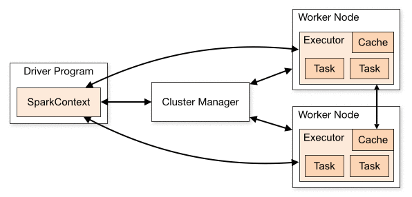
Image Credit: Apache Spark Docs
Spark provides an abstraction to work with a distributed dataset, the Resilient Distributed Dataset (RDD). RDD is an immutable distributed collection of objects partitioned across the cluster that can be operated on in parallel. RDDs can be created either by parallelizing a collection or an external dataset.
At a high level, the pipeline of our distributed inference application looks like this:

Spark by default creates one task per core on the executor. Since MXNet has built-in parallelism to efficiently use all the CPU cores, we’ll configure our application to create only one task per executor and let MXNet use all the cores on the instance. In the following code we will set the configuration key spark.executor.cores to 1, and pass the conf object when creating SparkContext. When submitting the application, you’ll see that we also set the number of executors to the number of workers available on the cluster. This forces one executor per node and turn off dynamic allocation of executors.
Load and partition data on the cluster
We have already copied CIFAR-10 data into an Amazon S3 bucket mxnet-spark-demo. Since the data stored in S3 can be accessed on all nodes we do not have to move data between the driver and executors. We will fetch only the S3 keys on the driver and create an RDD of keys using the boto library, which is the Python interface to access AWS services. This RDD will be partitioned and distributed to the executors in the cluster and we will fetch and process the mini-batch of images directly on the executors.
We will use the helper method fetch_s3_keys from utils.py to get all the keys from an Amazon S3 bucket. This method also takes a prefix to list keys that start with that prefix. The arguments are passed when you submit the main application.
The batch size as determined by args['batch'] is the number of images that can be fetched, preprocessed and run inference on each executor at once. This is bound by how much memory is available for each task. args['access_key'] and args['secret_key'] are optional arguments to access the S3 bucket in another account if Instance Role is set up with the right permissions. The script will automatically use the IAM role that was assigned to the cluster at launch.
We will split the RDD of keys into partitions with each partition containing a mini-batch of image keys. If the keys can’t be perfectly divided into partitions of batch size, we will fill the last partition to reuse some of the initial set of keys. This is needed since we will be binding (see the following code) to a fixed batch size.
Fetch and load data into Spark executors
In Apache Spark, you can perform two types of operations on RDDs. Transformation operates on the data in one RDD and creates a new RDD, and Action computes results on an RDD.
Transformations on RDDs are lazily evaluated. That is, Spark will not execute the transformations until it sees an action, instead, Spark keeps track of the dependencies between different RDDs by creating a directed acyclic graph that lead up to the action to form an execution plan. This helps in computing RDDs on demand and in recovery in case of a partition of the RDD is lost.
We’ll use Spark’s mapPartitions, which provides an iterator to the records of the partition. The transformation method is run separately on each partition (block) of the RDD. We will use the download_objects method from utils.py as the transformation on the RDD partition to download all the images of the partition from Amazon S3 into memory.
We’ll run another transformation to transform the each image in memory into a numpy array object using Python Pillow – Python Imaging Library. We’ll use Pillow to decode the images (in png format) in memory and translate to a numpy object. This is done in the read_images and load_images of mxinfer.py.
Note: In this application, you will see that we are importing the modules (numpy, mxnet, pillow, etc.,) inside the mapPartitions function instead of once at the top of the file. This is because PySpark will try to serialize all the modules and any dependent libraries that are imported at the module level and most often fail pickling the modules and any other associated binaries of the module. Otherwise Spark will expect that the routines and libraries are available on the nodes. We will ship the routines as code files when we submit the application using spark-submit script. The libraries are already installed on all the nodes. One more thing to look out for is if you use a member of an object in your function, Spark could end up serializing the entire object.
Inference using MXNet on the Executors
As stated earlier we will be running one executor per node and one task per executor for this application.
Before running inference, we have to load the model files. The MXModel class in mxinfer.py downloads the model files from MXNet model zoo and creates an MXNet module and stores it in the MXModel class at first use. We implemented a singleton pattern so that we do not have to instantiate and load the model for every prediction.
The download_model_files method in the MXModel singleton class will download the ResNet-18 model files. The model consists of a Symbol file with a .json extension that describes the neural network graph and a binary file with a .params extension containing the model parameters. For classification models, there will be a synsets.txt containing the classes and their corresponding labels.
After downloading the model files, we will load them and instantiate the MXNet module object in the init_module routine that performs the following steps:
- Load the symbol file and create a input Symbol, load parameters into an MXNet NDArray and parse arg_params and aux_params.
- Create a new MXNet module and assign the symbol.
- Bind symbol to input data.
- Set model parameters.
We will download and instantiate the MXModel object once on the first call to the predict method. The predict transformation method also takes a 4-dimensional array holding a batch (of size args['batch']) of color images (the other 3 dimensions of RGB) and calls the MXNet module forward method to produce the predictions for that batch of images.
Note: We are importing the mxnet and numpy modules within this method for the reasons discussed in the previous note.
Running the Inference Spark Application
First clone the deeplearning-emr GitHub repository that contain the codes for running inference using MXNet and Spark.
We will use the spark-submit script to run our Spark application.
Note: Replace <YOUR_S3_BUCKET> with the Amazon S3 bucket in which you want to store the result. You should have either a pass access/secret key or have permission in the Instance IAM role.
The arguments to the spark-submit are:
- --py-files: Comma separated list of code files (without spaces) that need to be shipped to the workers.
- --deploy-mode: cluster or client. When you run the application in cluster mode, Spark will choose one of the workers to run the driver and the executor. Running in cluster mode is useful when the cluster is of large size and the master node on the EMR cluster is busy running webservers for Hadoop, Spark, etc., You could also run the application in the client deploy mode.
- --master: yarn. EMR configures YARN as the resource manager.
- --conf spark.executor.memory Amount of memory that can used by each executor.
- --conf spark.executorEnv.LD_LIBRARY_PATH and --driver-library-path: set to LD_LIBRARY_PATH
- --num-executors: Total number of core and task nodes in the EMR cluster.
- infer_main.py: is the main program that starts the Spark application and it takes arguments S3 bucket, S3 key prefix, batch size, etc.
- --batch: Number of images that can be processed at a time on each executor. This is bound by the memory and CPU available on each worker node.
Collect predictions
Finally, we will collect the predictions generated for each partition using the Spark collect action and write those predictions to Amazon S3. The S3 location (args['output_s3_bucket'], args['output_s3_key']) to which results should be written can be passed as an argument to the infer_main.py.
Monitoring the Spark Application
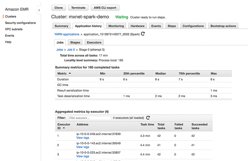
You can view the Spark application history and YARN application status right in the Amazon EMR console. The application history is updated throughout runtime in near real-time, and the history is available for up to seven days after the application is complete even after you have terminated the cluster. It also provides advanced metrics like memory usage, S3 reads, HDFS utilization, etc., all in one place. This also eliminates the need for SSH forwarding unlike when you use the YARN UI. You can find the features and how to use them in Spark Application History on EMR Console.
The following screenshot from the EMR console Application History shows the application tasks, execution times, etc.
Spark applications running on Amazon EMR can also be monitored using the Yarn ResourceManager Web UI on port 8088 on the driver host. The various web UIs available on the Amazon EMR cluster and how to access them are listed here: YARN Web UI on EMR.
The following screenshot illustrates the web monitoring tool. We can see the execution timeline, job duration, and task success and failures.

Another great feature of Amazon EMR is the integration with Amazon CloudWatch, which allows monitoring of cluster resources and applications. In the following screenshot below we can see the CPU utilization across the cluster nodes, which stayed below 25%.

Conclusion
To summarize, we demonstrated setting up a Spark cluster of 4 nodes, that uses MXNet to run distributed inference across 10000 images stored on Amazon S3, completing the processing within 5 (4.4) minutes.
Learn more
- Amazon Elastic MapReduce
- Apache Spark – Lightning-fast cluster computing
- Apache MXNet – Flexible and efficient deep learning.
- MXNet Symbol – Neural network graphs and auto-differentiation
- MXNet Module – Neural network training and inference
- MXNet – Using pre-trained models
- Spark Cluster Overview
- Submitting Spark Applications
Future improvements
- Compute/IO access optimization – In this application we have observed that the Compute/IO access on the executors has a square wave pattern where IO (no compute) and compute (no IO) are alternating. Ideally, this can be optimized by interleaving IO with compute. However, since we are using only one executor on each node it becomes challenging to manually manage resource utilization on each node.
- Using GPUs: Another big improvement would be to use GPUs to run inference on the batch of data.
About the Author
 Naveen Swamy is a Software Developer at Amazon AI working towards building innovative deep learning tools. His focus is to make deep learning accessible to software engineers to leverage their skills and apply them to everyday applications. In his spare time, he likes to spend time with his family.