리소스 센터 시작하기 / 10분 자습서 / ...
기계 학습 모델을 구축, 훈련, 배포 및 모니터링
(Amazon SageMaker Studio 사용)
Amazon SageMaker Studio는 최초의 완전 통합형 기계 학습 개발 환경(IDE)으로서, 모든 ML 개발 단계를 수행할 수 있는 단일 웹 기반 시각적 인터페이스를 제공합니다.
이 자습서에서는 Amazon SageMaker Studio를 사용하여 XGBoost 모델을 구축, 훈련, 배포 및 모니터링합니다. 기능 엔지니어링 및 모델 훈련에서부터 ML 모델의 배치 및 라이브 배포에 이르기까지 전체 기계 학습(ML) 워크플로를 다룹니다.
이 자습서에서는 다음 작업을 수행하는 방법을 알아봅니다.
- Amazon SageMaker Studio 제어판 설정
- Amazon SageMaker Studio 노트북으로 퍼블릭 데이터 세트를 다운로드하여 Amazon S3에 업로드
- Amazon SageMaker 실험을 생성하여 훈련 및 처리 작업을 추적 및 관리
- Amazon SageMaker 처리 작업을 실행하여 원시 데이터로 기능을 생성
- 내장 XGBoost 알고리즘을 사용하여 모델 훈련
- Amazon SageMaker 배치 변환을 사용하여 테스트 데이터 세트에서 모델 성능 테스트
- 모델을 엔드포인트로 배포하고 모니터링 작업을 설정하여 프로덕션에서 모델 엔드포인트의 데이터 드리프트를 모니터링합니다.
- SageMaker Model Monitor를 사용하여 결과를 시각화하고 모델을 모니터링함으로써 훈련 데이터 세트와 배포된 모델 간의 차이점을 확인합니다.
고객 인구 통계, 결제 내역 및 청구 내역에 대한 정보가 포함된 UCI 신용 카드 기본값 데이터 세트에 대해 모델을 훈련합니다.
| 자습서 소개 | |
|---|---|
| 시간 | 1시간 |
| 요금 | 10 USD 미만 |
| 사용 사례 | Machine Learning |
| 제품 | Amazon SageMaker |
| 대상 | 개발자, 데이터 사이언티스트 |
| 레벨 | 중급자용 |
| 최종 업데이트 날짜 | 2020년 8월 17일 |
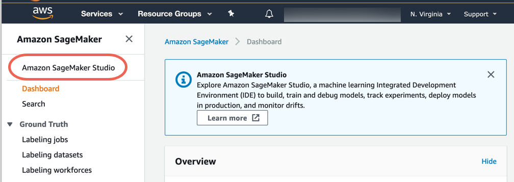
2단계. Amazon SageMaker Studio 제어판 생성
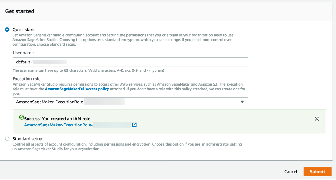
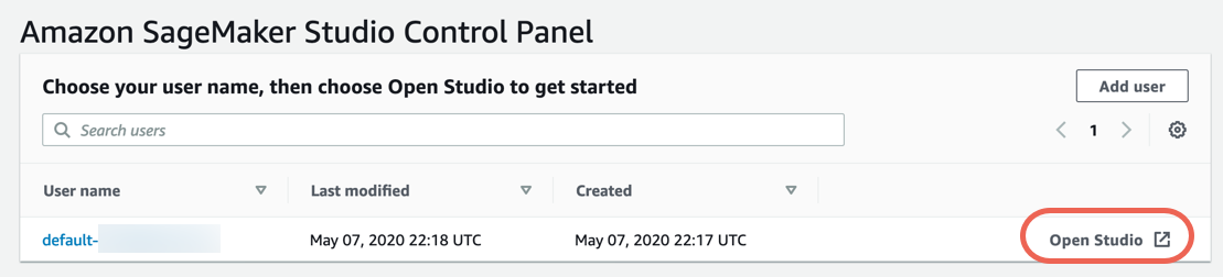
다음 단계에 따라 Amazon SageMaker Studio에 온보딩하여 Amazon SageMaker Studio 제어판을 설정합니다.
참고: 자세한 내용은 Amazon SageMaker 설명서에서 Amazon SageMaker Studio 시작하기를 참조하세요.
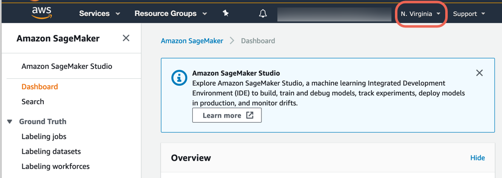
a. Amazon SageMaker 콘솔에 로그인합니다.
참고: 콘솔 오른쪽 위에서 SageMaker Studio를 사용할 수 있는 AWS 리전을 선택해야 합니다. 리전 목록은 Amazon SageMaker Studio에 온보딩을 참조하세요.
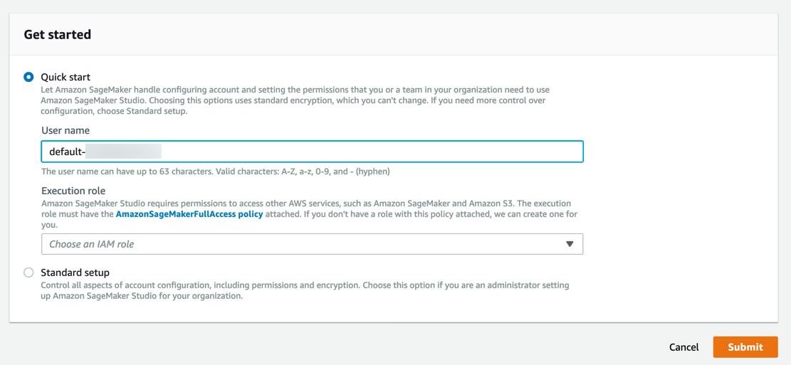
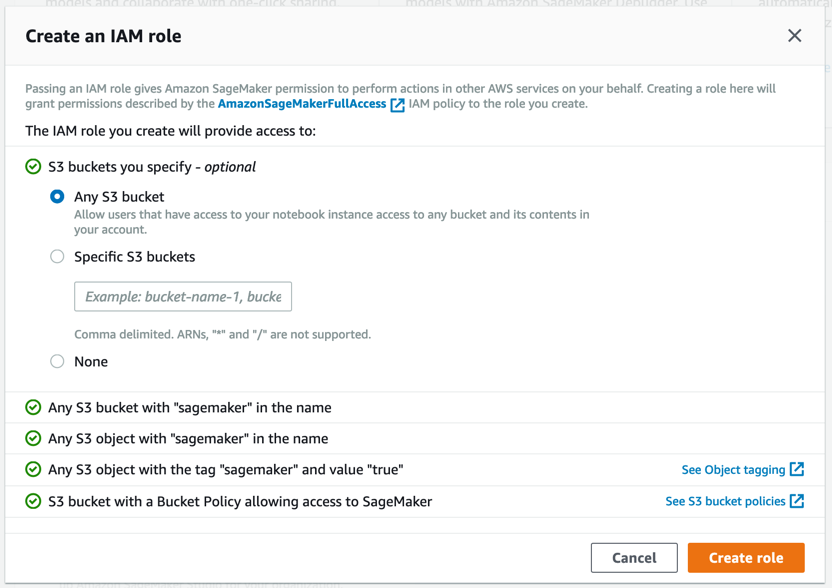
Amazon SageMaker에서 필요한 권한이 있는 역할이 생성되어 인스턴스에 할당됩니다.
3단계. 데이터 세트 다운로드
Amazon SageMaker Studio 노트북은 훈련 스크립트를 구축 및 테스트하는 데 필요한 모든 것이 포함된 원 클릭 Jupyter 노트북입니다. SageMaker Studio는 또한 실험 추적 및 시각화 기능도 갖추고 있어서 전체 기계 학습 워크플로를 한곳에서 편리하게 관리할 수 있습니다.
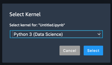
다음 단계를 수행하여 SageMaker 노트북을 생성하고 데이터 세트를 다운로드한 후에 Amazon S3에 업로드합니다.
참고: 자세한 내용은 Amazon SageMaker 설명서에서 Amazon SageMaker Studio 노트북 사용을 참조하세요.
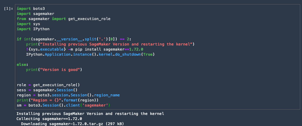
import boto3
import sagemaker
from sagemaker import get_execution_role
import sys

if int(sagemaker.__version__.split('.')[0]) == 2:
    !{sys.executable} -m pip install sagemaker==1.72.0
    print("Installing previous SageMaker Version. Please restart the kernel")
else:
    print("Version is good")

role = get_execution_role()
sess = sagemaker.Session()
region = boto3.session.Session().region_name
print("Region = {}".format(region))
sm = boto3.Session().client('sagemaker')
import matplotlib.pyplot as plt
import numpy as np
import pandas as pd
import os
from time import sleep, gmtime, strftime
import json
import time
!pip install sagemaker-experiments
from sagemaker.analytics import ExperimentAnalytics
from smexperiments.experiment import Experiment
from smexperiments.trial import Trial
from smexperiments.trial_component import TrialComponent
from smexperiments.tracker import Tracker
rawbucket= sess.default_bucket() # Alternatively you can use our custom bucket here.

prefix = 'sagemaker-modelmonitor' # use this prefix to store all files pertaining to this workshop.

dataprefix = prefix + '/data'
traindataprefix = prefix + '/train_data'
testdataprefix = prefix + '/test_data'
testdatanolabelprefix = prefix + '/test_data_no_label'
trainheaderprefix = prefix + '/train_headers'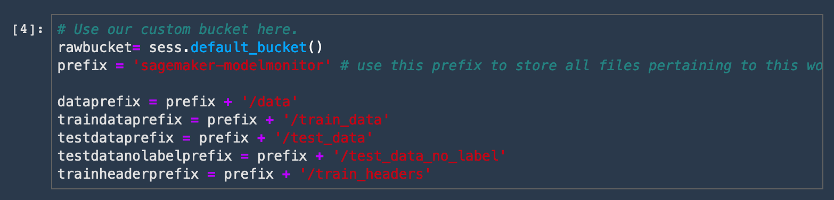
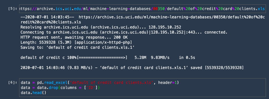
e. pandas 라이브러리를 통해 데이터 세트를 다운로드하여 가져옵니다. 다음 코드를 복사하여 새 코드 셀에 붙여넣고 [실행(Run)]을 선택합니다.
! wget https://archive.ics.uci.edu/ml/machine-learning-databases/00350/default%20of%20credit%20card%20clients.xls
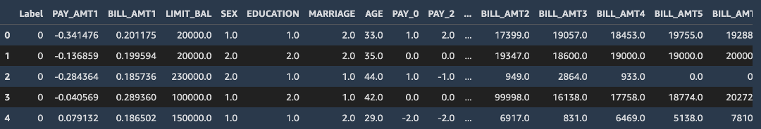
data = pd.read_excel('default of credit card clients.xls', header=1)
data = data.drop(columns = ['ID'])
data.head()
f. 마지막 열의 이름을 레이블로 바꾸고 레이블 열을 별도로 추출합니다. Amazon SageMaker 내장 XGBoost 알고리즘의 경우에 레이블 열은 데이터 프레임의 첫 번째 열이어야 합니다. 변경하려면 다음 코드를 복사하여 새 코드 셀에 붙여넣고 [실행(Run)]을 선택합니다.
data.rename(columns={"default payment next month": "Label"}, inplace=True)
lbl = data.Label
data = pd.concat([lbl, data.drop(columns=['Label'])], axis = 1)
data.head()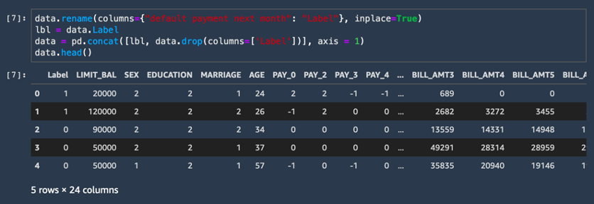
g. CSV 데이터 세트를 Amazon S3 버킷에 업로드합니다. 다음 코드를 복사하여 새 코드 셀에 붙여넣고 [실행(Run)]을 선택합니다.
if not os.path.exists('rawdata/rawdata.csv'):
    !mkdir rawdata
    data.to_csv('rawdata/rawdata.csv', index=None)
else:
    pass
# Upload the raw dataset
raw_data_location = sess.upload_data('rawdata', bucket=rawbucket, key_prefix=dataprefix)
print(raw_data_location)이제 작업이 완료되었습니다! 코드 출력에 다음 예시와 같은 S3 버킷 URI가 표시됩니다.
s3://sagemaker-us-east-2-ACCOUNT_NUMBER/sagemaker-modelmonitor/data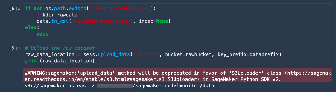
4 단계: Amazon SageMaker Processing을 사용하여 데이터 처리
이 단계에서는 Amazon SageMaker Processing을 사용하여 열의 크기를 조정하고 데이터 세트를 훈련 및 테스트 데이터로 분할하는 등, 데이터 세트를 전처리합니다. SageMaker Processing은 완전 관리형 인프라에서 전처리, 후처리 및 모델 평가 워크로드를 쉽게 실행할 수 있습니다.
Amazon SageMaker Processing에서 다음 단계를 통해 데이터를 처리하고 기능을 생성하세요.
참고: Amazon SageMaker Processing은 노트북과 별도의 컴퓨팅 인스턴스에서 실행할 수 있습니다. 이는 처리 작업이 진행되는 동안 노트북에서 코드를 계속 실험하면서 실행할 수 있다는 것을 의미합니다. 따라서 처리 작업 기간 동안 실행하는 인스턴스 비용에 대한 추가 요금이 발생합니다. 처리 작업이 완료되면 SageMaker가 인스턴스를 자동으로 종료합니다. 자세한 요금은 Amazon SageMaker 요금 페이지를 참조하세요.
참고: 자세한 내용은 Amazon SageMaker 설명서의 데이터 처리 및 모델 평가를 참조하세요.
a. scikit-learn processing 컨테이너를 가져옵니다. 다음 코드를 복사하여 새 코드 셀에 붙여넣고 [실행(Run)]을 선택합니다.
참고: Amazon SageMaker는 scikit-learn에 관리형 컨테이너를 제공합니다. 자세한 내용은 scikit-learn을 사용한 데이터 처리 및 모델 평가를 참조하세요.
from sagemaker.sklearn.processing import SKLearnProcessor
sklearn_processor = SKLearnProcessor(framework_version='0.20.0',
                                     role=role,
                                     instance_type='ml.c4.xlarge',
                                     instance_count=1)
b. 다음 전처리 스크립트를 복사하여 새 셀에 붙여넣고 [실행(Run)]을 선택합니다.
%%writefile preprocessing.py

import argparse
import os
import warnings

import pandas as pd
import numpy as np
from sklearn.model_selection import train_test_split
from sklearn.preprocessing import StandardScaler, MinMaxScaler
from sklearn.exceptions import DataConversionWarning
from sklearn.compose import make_column_transformer

warnings.filterwarnings(action='ignore', category=DataConversionWarning)

if __name__=='__main__':
    parser = argparse.ArgumentParser()
    parser.add_argument('--train-test-split-ratio', type=float, default=0.3)
    parser.add_argument('--random-split', type=int, default=0)
    args, _ = parser.parse_known_args()

    print('Received arguments {}'.format(args))

    input_data_path = os.path.join('/opt/ml/processing/input', 'rawdata.csv')

    print('Reading input data from {}'.format(input_data_path))
    df = pd.read_csv(input_data_path)
    df.sample(frac=1)

    COLS = df.columns
    newcolorder = ['PAY_AMT1','BILL_AMT1'] + list(COLS[1:])[:11] + list(COLS[1:])[12:17] + list(COLS[1:])[18:]

    split_ratio = args.train_test_split_ratio
    random_state=args.random_split

    X_train, X_test, y_train, y_test = train_test_split(df.drop('Label', axis=1), df['Label'],
                                                        test_size=split_ratio, random_state=random_state)

    preprocess = make_column_transformer(
        (['PAY_AMT1'], StandardScaler()),
        (['BILL_AMT1'], MinMaxScaler()),
    remainder='passthrough')

    print('Running preprocessing and feature engineering transformations')
    train_features = pd.DataFrame(preprocess.fit_transform(X_train), columns = newcolorder)
    test_features = pd.DataFrame(preprocess.transform(X_test), columns = newcolorder)

    # concat to ensure Label column is the first column in dataframe
    train_full = pd.concat([pd.DataFrame(y_train.values, columns=['Label']), train_features], axis=1)
    test_full = pd.concat([pd.DataFrame(y_test.values, columns=['Label']), test_features], axis=1)

    print('Train data shape after preprocessing: {}'.format(train_features.shape))
    print('Test data shape after preprocessing: {}'.format(test_features.shape))

    train_features_headers_output_path = os.path.join('/opt/ml/processing/train_headers', 'train_data_with_headers.csv')

    train_features_output_path = os.path.join('/opt/ml/processing/train', 'train_data.csv')

    test_features_output_path = os.path.join('/opt/ml/processing/test', 'test_data.csv')

    print('Saving training features to {}'.format(train_features_output_path))
    train_full.to_csv(train_features_output_path, header=False, index=False)
    print("Complete")

    print("Save training data with headers to {}".format(train_features_headers_output_path))
    train_full.to_csv(train_features_headers_output_path, index=False)

    print('Saving test features to {}'.format(test_features_output_path))
    test_full.to_csv(test_features_output_path, header=False, index=False)
print("Complete")c. 다음 코드를 사용하여 전처리 코드를 Amazon S3 버킷에 복사한 후에 [실행(Run)]을 선택합니다.
# Copy the preprocessing code over to the s3 bucket
codeprefix = prefix + '/code'
codeupload = sess.upload_data('preprocessing.py', bucket=rawbucket, key_prefix=codeprefix)
print(codeupload)

d. SageMaker 처리 작업이 완료된 후에 훈련 및 테스트 데이터를 저장할 위치를 지정합니다. Amazon SageMaker Processing가 데이터를 지정된 위치에 자동으로 저장합니다.
train_data_location = rawbucket + '/' + traindataprefix
test_data_location = rawbucket+'/'+testdataprefix
print("Training data location = {}".format(train_data_location))
print("Test data location = {}".format(test_data_location))
e. 처리 작업을 시작하려면 다음 코드를 복사하여 붙여넣습니다. 이 코드가 sklearn_processor.run을 호출하여 작업을 시작하면서 훈련 및 테스트 출력이 저장된 위치 등, 처리 작업에 대한 일부 선택적 메타데이터를 추출합니다.
from sagemaker.processing import ProcessingInput, ProcessingOutput

sklearn_processor.run(code=codeupload,
                      inputs=[ProcessingInput(
                        source=raw_data_location,
                        destination='/opt/ml/processing/input')],
                      outputs=[ProcessingOutput(output_name='train_data',
                                                source='/opt/ml/processing/train',
                               destination='s3://' + train_data_location),
                               ProcessingOutput(output_name='test_data',
                                                source='/opt/ml/processing/test',
                                               destination="s3://"+test_data_location),
                               ProcessingOutput(output_name='train_data_headers',
                                                source='/opt/ml/processing/train_headers',
                                               destination="s3://" + rawbucket + '/' + prefix + '/train_headers')],
                      arguments=['--train-test-split-ratio', '0.2']
                     )

preprocessing_job_description = sklearn_processor.jobs[-1].describe()

output_config = preprocessing_job_description['ProcessingOutputConfig']
for output in output_config['Outputs']:
    if output['OutputName'] == 'train_data':
        preprocessed_training_data = output['S3Output']['S3Uri']
    if output['OutputName'] == 'test_data':
        preprocessed_test_data = output['S3Output']['S3Uri']
프로세서에 제공되는 출력에서 코드, 훈련 및 테스트 데이터의 위치에 유의합니다. 또한 처리 스크립트에 제공되는 인수에도 유의합니다.

5 단계: Amazon SageMaker 실험 생성
이제 Amazon S3에서 데이터 세트를 다운로드하고 스테이징했으므로 Amazon SageMaker 실험을 생성할 수 있습니다. 실험은 같은 기계 학습 프로젝트와 관련된 처리 및 훈련 작업의 모음입니다. Amazon SageMaker 실험은 훈련 실행을 자동으로 관리하고 추적합니다.
다음 단계에 따라 새 실험을 생성합니다.
참고: 자세한 내용은 Amazon SageMaker 설명서의 실험을 참조하세요.
a. 다음 코드를 복사하고 붙여넣어 Build-train-deploy-라는 실험을 생성합니다.
# Create a SageMaker Experiment
cc_experiment = Experiment.create(
    experiment_name=f"Build-train-deploy-{int(time.time())}",
    description="Predict credit card default from payments data",
    sagemaker_boto_client=sm)
print(cc_experiment)
모든 훈련 작업은 평가판으로 기록됩니다. 각 평가판은 종단간 훈련 작업의 반복입니다. 훈련 작업 이외에도 데이터 세트 및 기타 메타데이터뿐만 아니라 전처리 및 후처리 작업을 추적할 수도 있습니다. 단일 실험은 Amazon SageMaker Studio 실험 창에서 시간 경과에 따라 여러 반복을 쉽게 추적할 수 있게 하는 여러 평가판을 포함할 수 있습니다.
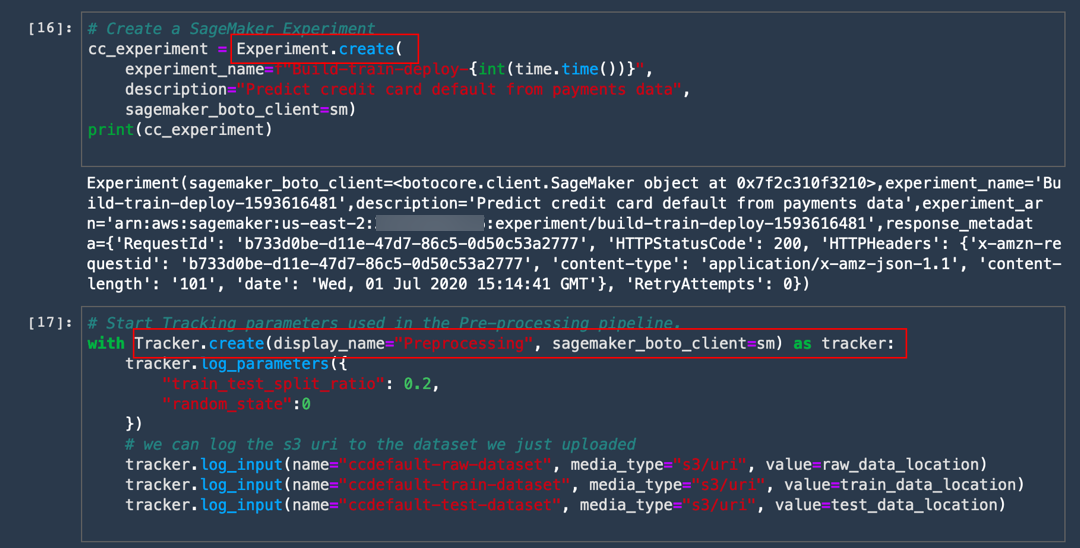
b. 다음 코드를 복사하고 붙여넣어 훈련 파이프라인의 단계뿐만 아니라 실험 아래의 전처리 작업도 추적합니다.
# Start Tracking parameters used in the Pre-processing pipeline.
with Tracker.create(display_name="Preprocessing", sagemaker_boto_client=sm) as tracker:
    tracker.log_parameters({
        "train_test_split_ratio": 0.2,
        "random_state":0
    })
    # we can log the s3 uri to the dataset we just uploaded
    tracker.log_input(name="ccdefault-raw-dataset", media_type="s3/uri", value=raw_data_location)
    tracker.log_input(name="ccdefault-train-dataset", media_type="s3/uri", value=train_data_location)
    tracker.log_input(name="ccdefault-test-dataset", media_type="s3/uri", value=test_data_location)
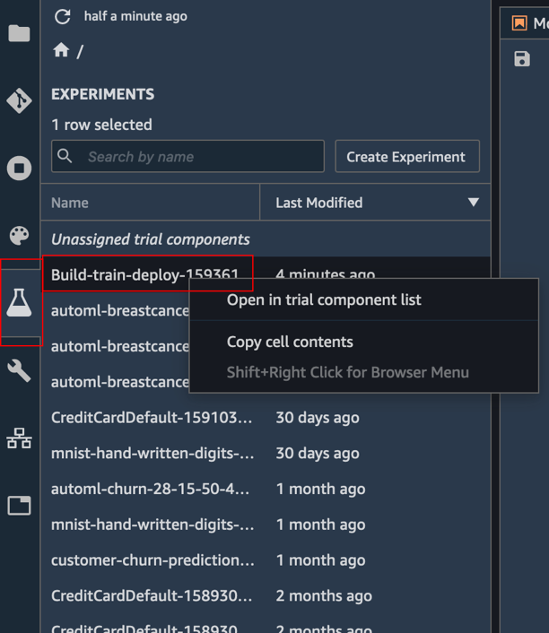
c. 실험 세부 정보 보기: 실험 창에서 Build-train-deploy-라는 실험을 마우스 오른쪽 버튼으로 클릭하여 [평가판 구성 요소 목록에서 열기(Open in trial components list)]를 선택합니다.
d. 다음 코드를 복사하여 붙여넣은 후에 [실행(Run)]을 선택합니다. 이제 코드를 자세히 살펴보겠습니다.
XGBoost 분류자를 훈련하려면 먼저 Amazon SageMaker에서 유지 관리하는 XGBoost 컨테이너를 가져옵니다. 그런 다음, SageMaker 실험에서 평가판 이름으로 추적할 수 있도록 훈련 실행을 평가판에 기록합니다. 전처리 작업은 파이프라인의 일부이므로 동일한 평가판 이름으로 포함됩니다. 다음, 선택한 기본 인스턴스 유형의 자동 프로비저닝, 훈련 데이터를 처리 작업의 지정된 출력 위치에서 복사, 모델 훈련, 모델 아티팩트 출력 등의 작업을 수행하는 SageMaker 추정기 객체를 생성합니다.
from sagemaker.amazon.amazon_estimator import get_image_uri
container = get_image_uri(boto3.Session().region_name, 'xgboost', '1.0-1')
s3_input_train = sagemaker.s3_input(s3_data='s3://' + train_data_location, content_type='csv')
preprocessing_trial_component = tracker.trial_component

trial_name = f"cc-default-training-job-{int(time.time())}"
cc_trial = Trial.create(
        trial_name=trial_name,
            experiment_name=cc_experiment.experiment_name,
        sagemaker_boto_client=sm
    )

cc_trial.add_trial_component(preprocessing_trial_component)
cc_training_job_name = "cc-training-job-{}".format(int(time.time()))

xgb = sagemaker.estimator.Estimator(container,
                                    role,
                                    train_instance_count=1,
                                    train_instance_type='ml.m4.xlarge',
                                    train_max_run=86400,
                                    output_path='s3://{}/{}/models'.format(rawbucket, prefix),
                                    sagemaker_session=sess) # set to true for distributed training

xgb.set_hyperparameters(max_depth=5,
                        eta=0.2,
                        gamma=4,
                        min_child_weight=6,
                        subsample=0.8,
                        verbosity=0,
                        objective='binary:logistic',
                        num_round=100)

xgb.fit(inputs = {'train':s3_input_train},
       job_name=cc_training_job_name,
        experiment_config={
            "TrialName": cc_trial.trial_name, #log training job in Trials for lineage
            "TrialComponentDisplayName": "Training",
        },
        wait=True,
    )
time.sleep(2)
훈련 작업은 완료하는 데 약 70초가 소요됩니다. 다음 출력을 볼 수 있어야 합니다.
Completed - Training job completed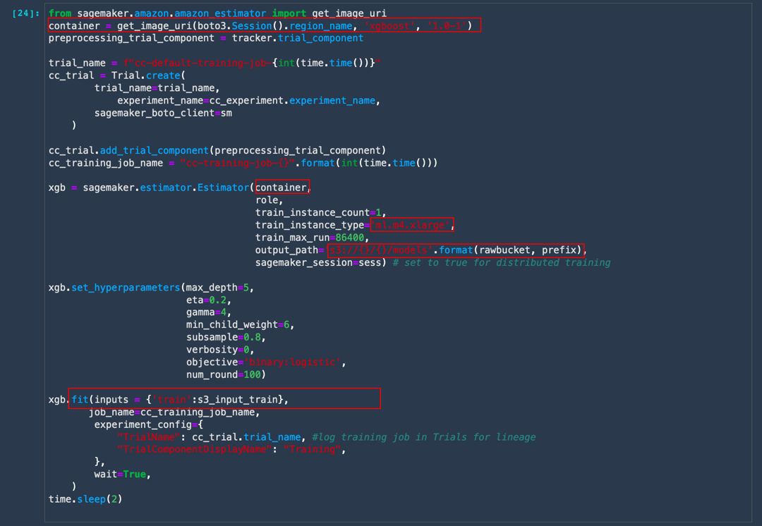
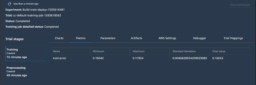
e. 왼쪽 도구 모음에서 [실험(Experiment)]을 선택합니다. Build-train-deploy- 실험을 마우스 오른쪽 버튼으로 클릭하고 [평가판 구성 요소 목록에서 열기(Open in trial components list)]를 선택합니다. Amazon SageMaker 실험에서 실패한 훈련 실행을 포함한 모든 실행을 캡처합니다.
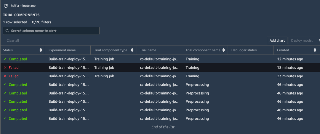
f. 완료된 훈련 작업 중 하나를 마우스 오른쪽 버튼으로 클릭하고 [평가판 세부 정보에서 열기(Open in Trial Details)]를 선택하여 훈련 작업에 관련된 메타데이터를 탐색합니다.
참고: 최신 결과를 보려면 페이지를 새로 고침해야 할 수 있습니다.
6단계: 오프라인 추론 모델 배포
전처리 단계에서 일부 테스트 데이터를 생성했습니다. 이 단계에서는 훈련된 모델에서 오프라인 또는 배치 추론을 생성하여 처음 보는 테스트 데이터에 대한 모델 성능을 평가합니다.
오프라인 추론 모델을 배포하려면 다음 단계를 수행합니다.
참고: 자세한 내용은 Amazon SageMaker 설명서에서 배치 변환을 참조하세요.
a. 다음 코드를 복사하여 붙여넣은 후에 [실행(Run)]을 선택합니다.
이 단계에서는 테스트 데이터 세트를 Amazon S3 위치에서 로컬 폴더로 복사합니다.
test_data_path = 's3://' + test_data_location + '/test_data.csv'
! aws s3 cp $test_data_path .
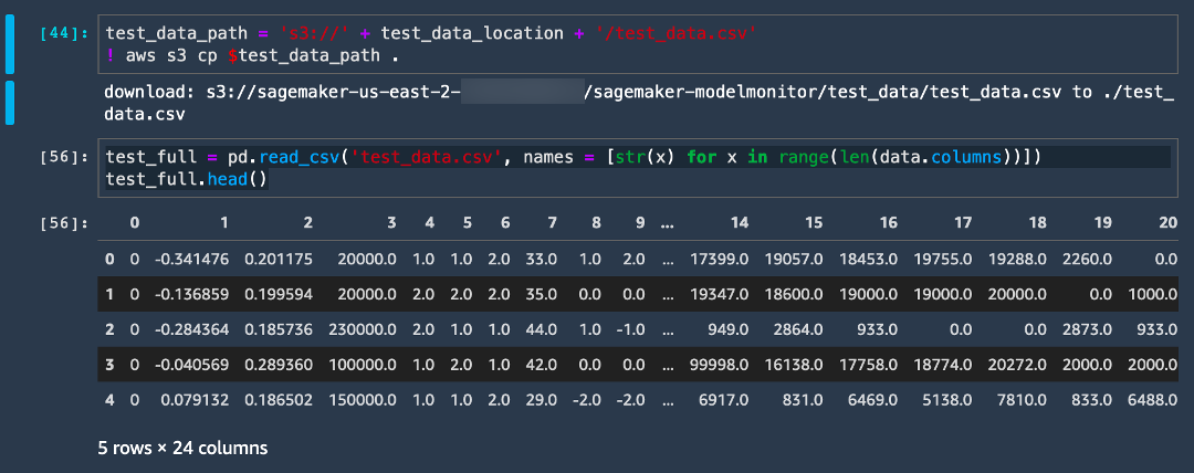
b. 다음 코드를 복사하여 붙여넣은 후에 [실행(Run)]을 선택합니다.
test_full = pd.read_csv('test_data.csv', names = [str(x) for x in range(len(data.columns))])
test_full.head()
c. 다음 코드를 복사하여 붙여넣은 후에 [실행(Run)]을 선택합니다. 이 단계에서는 레이블 열을 추출합니다.
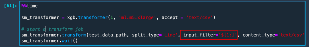
label = test_full['0'] d. 다음 코드를 복사하여 붙여넣고 [실행(Run)]을 선택하여 배치 변환 작업을 생성합니다. 이제 코드를 자세히 살펴보겠습니다.
훈련 작업과 마찬가지로 SageMaker가 모든 기본 리소스를 프로비저닝하고 훈련된 모델 아티팩트를 복사하며, 배치 엔드포인트를 로컬로 설정하고 데이터를 복사하며, 데이터에 대한 추론을 실행하고 출력을 Amazon S3으로 푸시합니다. input_filter를 설정하면 배치 변환에 레이블 열인 테스트 데이터에서 첫 번째 열을 무시하도록 알릴 수 있습니다.
%%time

sm_transformer = xgb.transformer(1, 'ml.m5.xlarge', accept = 'text/csv')

# start a transform job
sm_transformer.transform(test_data_path, split_type='Line', input_filter='$[1:]', content_type='text/csv')
sm_transformer.wait()
배치 변환 작업은 완료하는 데 약 4분이 소요되며, 이후에 모델 결과를 평가할 수 있습니다.
e. 다음 코드를 복사 및 실행하여 모델 지표를 평가합니다. 이제 코드를 자세히 살펴보겠습니다.
먼저 확장명이 .out인 파일에 포함된 배치 변환 작업의 출력을 Amazon S3 버킷에서 가져오기 위한 함수를 정의합니다. 그런 다음, 예측된 레이블을 데이터 프레임으로 추출하고 실제 레이블을 이 데이터 프레임에 추가합니다.
import json
import io
from urllib.parse import urlparse
def get_csv_output_from_s3(s3uri, file_name):
parsed_url = urlparse(s3uri)
bucket_name = parsed_url.netloc
prefix = parsed_url.path[1:]
s3 = boto3.resource('s3')
obj = s3.Object(bucket_name, '{}/{}'.format(prefix, file_name))
return obj.get()["Body"].read().decode('utf-8')
output = get_csv_output_from_s3(sm_transformer.output_path, 'test_data.csv.out')
output_df = pd.read_csv(io.StringIO(output), sep=",", header=None)
output_df.head(8)
output_df['Predicted']=np.round(output_df.values)
output_df['Label'] = label
from sklearn.metrics import confusion_matrix, accuracy_score
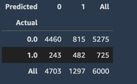
confusion_matrix = pd.crosstab(output_df['Predicted'], output_df['Label'], rownames=['Actual'], colnames=['Predicted'], margins = True)
confusion_matrix
예측 참 및 거짓 값의 합계를 실제 값과 비교하여 표시하는 이미지와 유사한 출력을 볼 수 있어야 합니다.
f. 다음 코드를 사용하여 기준 모델 정확도와 모델 정확도를 모두 추출합니다.
참고: 기준 정확도에 유용한 모델은 기본 사례 이외의 사례일 수도 있습니다. 사용자가 기본값이 아니라고 항상 예측하는 모델은 이 정확도를 가집니다.
print("Baseline Accuracy = {}".format(1- np.unique(data['Label'], return_counts=True)[1][1]/(len(data['Label']))))
print("Accuracy Score = {}".format(accuracy_score(label, output_df['Predicted'])))
결과는 단순 모델이 이미 기준 정확도를 상회할 수 있음을 보여줍니다. 결과를 개선하려면 하이퍼파라미터를 튜닝할 수 있습니다. SageMaker에서 하이퍼파라미터 최적화(HPO)를 사용하여 자동 모델 튜닝을 수행할 수 있습니다. 자세한 내용은 하이퍼파라미터 튜닝 작동 방식을 참조하세요.
참고: 이 자습서에서는 다루지 않지만 배치 변환을 평가판의 일부로 포함시키는 옵션도 사용할 수 있습니다. 훈련 작업에서와 마찬가지로 .transform 함수를 호출할 때 experiment_config를 전달하기만 하면 됩니다. Amazon SageMaker가 평가판 구성 요소로서 배치 변환을 자동 연결합니다.

7단계: 모델을 엔드포인트로 배포하고 데이터 캡처 설정
이 단계에서는 모델을 RESTful HTTPS 엔드포인트로 배포하여 라이브 추론을 제공합니다. Amazon SageMaker는 모델 호스팅 및 엔드포인트 생성을 자동으로 처리합니다.
다음 단계를 수행하여 모델을 엔드포인트로 배포하고 데이터 캡처를 설정합니다.
참고: 자세한 내용은 Amazon SageMaker 설명서의 추론 모델 배포를 참조하세요.
a. 다음 코드를 복사하여 붙여넣은 후에 [실행(Run)]을 선택합니다.
from sagemaker.model_monitor import DataCaptureConfig
from sagemaker import RealTimePredictor
from sagemaker.predictor import csv_serializer

sm_client = boto3.client('sagemaker')

latest_training_job = sm_client.list_training_jobs(MaxResults=1,
                                                SortBy='CreationTime',
                                                SortOrder='Descending')

training_job_name=TrainingJobName=latest_training_job['TrainingJobSummaries'][0]['TrainingJobName']

training_job_description = sm_client.describe_training_job(TrainingJobName=training_job_name)

model_data = training_job_description['ModelArtifacts']['S3ModelArtifacts']
container_uri = training_job_description['AlgorithmSpecification']['TrainingImage']

# create a model.
def create_model(role, model_name, container_uri, model_data):
    return sm_client.create_model(
        ModelName=model_name,
        PrimaryContainer={
        'Image': container_uri,
        'ModelDataUrl': model_data,
        },
        ExecutionRoleArn=role)


try:
    model = create_model(role, training_job_name, container_uri, model_data)
except Exception as e:
        sm_client.delete_model(ModelName=training_job_name)
        model = create_model(role, training_job_name, container_uri, model_data)


print('Model created: '+model['ModelArn'])

b. 데이터 구성 설정을 지정하려면 다음 코드를 복사하여 붙여넣은 후에 [실행(Run)]을 선택합니다.
이 코드는 SageMaker에 엔드포인트에서 수신한 추론 페이로드를 100% 캡처하고 입출력을 모두 캡처하며 입력 콘텐츠 유형을 csv로 기록하도록 지시합니다.
s3_capture_upload_path = 's3://{}/{}/monitoring/datacapture'.format(rawbucket, prefix)
data_capture_configuration = {
    "EnableCapture": True,
    "InitialSamplingPercentage": 100,
    "DestinationS3Uri": s3_capture_upload_path,
    "CaptureOptions": [
        { "CaptureMode": "Output" },
        { "CaptureMode": "Input" }
    ],
    "CaptureContentTypeHeader": {
       "CsvContentTypes": ["text/csv"],
       "JsonContentTypes": ["application/json"]}
c. 다음 코드를 복사하여 붙여넣은 후에 [실행(Run)]을 선택합니다. 이 단계에서는 엔드포인트 구성을 생성하여 엔드포인트를 배포합니다. 코드에서 인스턴스 유형과 모든 트래픽을 이 엔드포인트로 전송할지 여부 등을 지정할 수 있습니다.
def create_endpoint_config(model_config, data_capture_config):
    return sm_client.create_endpoint_config(
                                                EndpointConfigName=model_config,
                                                ProductionVariants=[
                                                        {
                                                            'VariantName': 'AllTraffic',
                                                            'ModelName': model_config,
                                                            'InitialInstanceCount': 1,
                                                            'InstanceType': 'ml.m4.xlarge',
                                                            'InitialVariantWeight': 1.0,
                                                },

                                                    ],
                                                DataCaptureConfig=data_capture_config
                                                )


try:
    endpoint_config = create_endpoint_config(training_job_name, data_capture_configuration)
except Exception as e:
    sm_client.delete_endpoint_config(EndpointConfigName=endpoint)
    endpoint_config = create_endpoint_config(training_job_name, data_capture_configuration)

print('Endpoint configuration created: '+ endpoint_config['EndpointConfigArn'])
d. 다음 코드를 복사하여 붙여넣은 후에 [실행(Run)]을 선택하여 엔드포인트를 생성합니다.
# Enable data capture, sampling 100% of the data for now. Next we deploy the endpoint in the correct VPC.

endpoint_name = training_job_name
def create_endpoint(endpoint_name, config_name):
    return sm_client.create_endpoint(
                                    EndpointName=endpoint_name,
                                    EndpointConfigName=training_job_name
                                )


try:
    endpoint = create_endpoint(endpoint_name, endpoint_config)
except Exception as e:
    sm_client.delete_endpoint(EndpointName=endpoint_name)
    endpoint = create_endpoint(endpoint_name, endpoint_config)

print('Endpoint created: '+ endpoint['EndpointArn'])

e. 왼쪽 도구 모음에서 [엔드포인트(Endpoints)]를 선택합니다. 엔드포인트 목록은 서비스 중인 모든 엔드포인트를 표시합니다.
build-train-deploy 엔드포인트가 생성 중(Creating) 상태를 표시하는지 확인합니다. 모델을 배포하려면 Amazon SageMaker가 먼저 모델 아티팩트 및 추론 이미지를 인스턴스에 복사하고 HTTPS 엔드포인트를 설정하여 클라이언트 애플리케이션 또는 RESTful API에 연결해야 합니다.
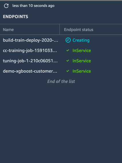
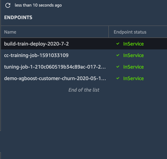
엔드포인트가 생성되면 상태가 서비스 중(InService)으로 변경됩니다. (엔드포인트 생성에는 약 5-10분이 소요될 수 있음에 유의합니다.)
참고: 업데이트된 상태를 보려면 새로 고침을 클릭해야 할 수 있습니다.
f. JupyterLab 노트북에서 다음 코드를 복사하고 실행하여 테스트 데이터 세트의 샘플을 취합니다. 이 코드는 처음 10개 행을 사용합니다.
!head -10 test_data.csv > test_sample.csvg. 다음 코드를 실행하여 추론 요청을 이 엔드포인트에 전송합니다.
참고: 다른 엔드포인트 이름을 지정한 경우 아래의 엔드포인트를 귀하의 엔드포인트 이름으로 변경해야 합니다.
from sagemaker import RealTimePredictor
from sagemaker.predictor import csv_serializer

predictor = RealTimePredictor(endpoint=endpoint_name, content_type = 'text/csv')

with open('test_sample.csv', 'r') as f:
    for row in f:
        payload = row.rstrip('\n')
        response = predictor.predict(data=payload[2:])
        sleep(0.5)
print('done!')
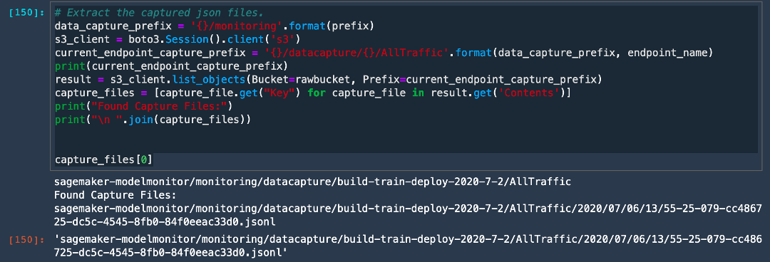
h. 다음 코드를 실행하여 모델 모니터가 수신 데이터를 올바르게 캡처하고 있는지 확인합니다.
코드에서 current_endpoint_capture_prefix는 ModelMonitor 출력이 저장되는 디렉터리 경로를 캡처합니다. Amazon S3 버킷으로 이동하여 예측 요청이 캡처되고 있는지 확인합니다. 이 위치가 위 코드의 s3_capture_upload_path와 일치해야 한다는 점에 유의합니다.
# Extract the captured json files.
data_capture_prefix = '{}/monitoring'.format(prefix)
s3_client = boto3.Session().client('s3')
current_endpoint_capture_prefix = '{}/datacapture/{}/AllTraffic'.format(data_capture_prefix, endpoint_name)
print(current_endpoint_capture_prefix)
result = s3_client.list_objects(Bucket=rawbucket, Prefix=current_endpoint_capture_prefix)
capture_files = [capture_file.get("Key") for capture_file in result.get('Contents')]
print("Found Capture Files:")
print("\n ".join(capture_files))


capture_files[0]
캡처된 출력이 데이터 캡처가 구성되어 수신 요청을 저장하고 있음을 나타냅니다.
참고: 처음에 Null 응답이 표시되는 경우, 데이터 캡처를 처음 초기화할 때 데이터가 Amazon S3 경로에 동기식으로 로드되지 않았을 수 있습니다. 1분 정도 기다린 후에 다시 시도하세요.
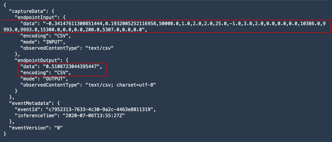
i. 다음 코드를 실행하여 json 파일 중 하나의 콘텐츠를 추출하고 캡처된 출력을 확인합니다.
# View contents of the captured file.
def get_obj_body(bucket, obj_key):
    return s3_client.get_object(Bucket=rawbucket, Key=obj_key).get('Body').read().decode("utf-8")

capture_file = get_obj_body(rawbucket, capture_files[0])
print(json.dumps(json.loads(capture_file.split('\n')[5]), indent = 2, sort_keys =True))
출력이 데이터 캡처가 모델의 입력 페이로드와 출력을 모두 캡처하고 있음을 나타냅니다.
8 단계: SageMaker Model Monitor로 엔드포인트 모니터링
이 단계에서는 SageMaker Model Monitor를 활성화하여 배포된 엔드포인트의 데이터 드리프트를 모니터링합니다. 이를 위해 모델에 전송된 페이로드와 출력을 기준과 비교하여 입력 데이터 또는 레이블에 드리프트가 발생했는지 확인합니다.
모델 모니터링을 활성화하려면 다음 단계를 완료하세요.
참고: 자세한 내용은 Amazon SageMaker 설명서의 Amazon SageMaker Model Monitor를 참조하세요.
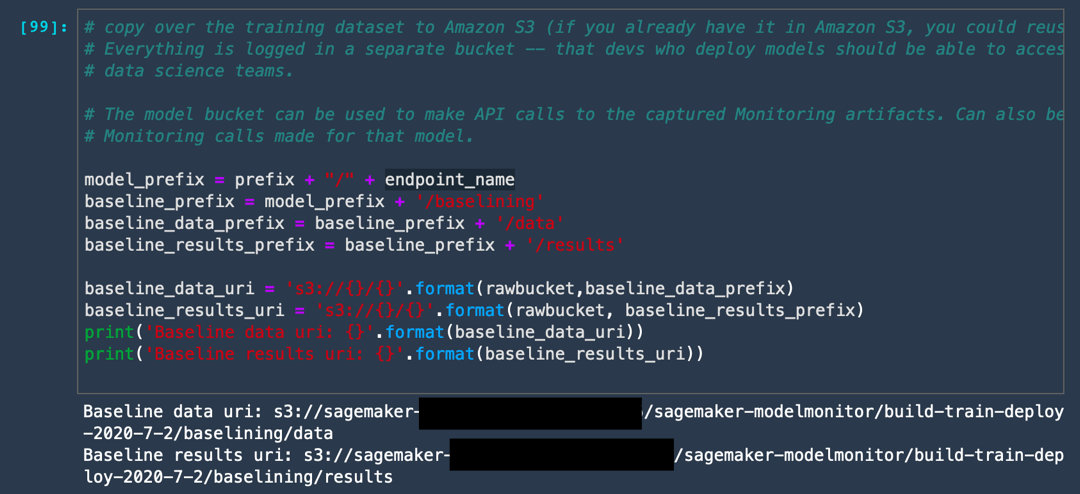
a. 다음 코드를 실행하여 Amazon S3 버킷에 Model Monitor의 출력을 저장할 폴더를 생성합니다.
이 코드는 두 개의 폴더를 생성합니다. 즉, 모델 훈련에 사용한 기준 데이터를 저장하는 폴더와 해당 기준의 모든 위반 사항을 저장하는 폴더입니다.
model_prefix = prefix + "/" + endpoint_name
baseline_prefix = model_prefix + '/baselining'
baseline_data_prefix = baseline_prefix + '/data'
baseline_results_prefix = baseline_prefix + '/results'

baseline_data_uri = 's3://{}/{}'.format(rawbucket,baseline_data_prefix)
baseline_results_uri = 's3://{}/{}'.format(rawbucket, baseline_results_prefix)
train_data_header_location = "s3://" + rawbucket + '/' + prefix + '/train_headers'
print('Baseline data uri: {}'.format(baseline_data_uri))
print('Baseline results uri: {}'.format(baseline_results_uri))
print(train_data_header_location)
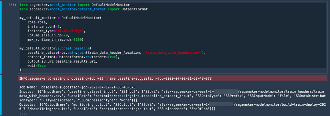
b. 다음 코드를 실행하여 훈련 데이터의 통계를 캡처하기 위한 Model Monitor의 기준 작업을 설정합니다. 이를 위해 Model Monitor는 Apache Spark 상에 구축된 deequ 라이브러리를 사용하여 데이터에 대한 단위 테스트를 수행합니다.
from sagemaker.model_monitor import DefaultModelMonitor
from sagemaker.model_monitor.dataset_format import DatasetFormat

my_default_monitor = DefaultModelMonitor(
    role=role,
    instance_count=1,
    instance_type='ml.m5.xlarge',
    volume_size_in_gb=20,
    max_runtime_in_seconds=3600)

my_default_monitor.suggest_baseline(
    baseline_dataset=os.path.join(train_data_header_location, 'train_data_with_headers.csv'),
    dataset_format=DatasetFormat.csv(header=True),
    output_s3_uri=baseline_results_uri,
    wait=True
)
Model Monitor가 별도의 인스턴스를 설정하고 훈련 데이터를 복사하며 일부 통계를 생성합니다. 이 서비스는 무시할 수 있는 많은 Apache Spark 로그를 생성합니다. 작업이 완료되면 Spark 작업 완료됨 출력을 볼 수 있습니다.
c. 다음 코드를 실행하여 기준 작업에서 생성된 출력을 확인합니다.
s3_client = boto3.Session().client('s3')
result = s3_client.list_objects(Bucket=rawbucket, Prefix=baseline_results_prefix)
report_files = [report_file.get("Key") for report_file in result.get('Contents')]
print("Found Files:")
print("\n ".join(report_files))
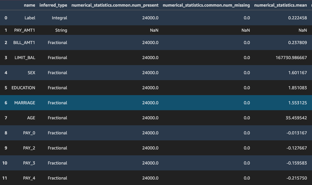
baseline_job = my_default_monitor.latest_baselining_job
schema_df = pd.io.json.json_normalize(baseline_job.baseline_statistics().body_dict["features"])
schema_df
constraints.json 및 statistics.json의 두 파일을 볼 수 있습니다. 다음에 그 내용을 세부적으로 확인합니다.
위의 코드가 /statistics.json의 json 출력을 pandas 데이터 프레임으로 변환합니다. deequ 라이브러리가 열의 데이터 유형, Null 또는 결측값의 유무 그리고 입력 데이터 스트림의 평균, 최소, 최대, 합계, 표준 편차 및 스케치 파라미터와 같은 통계 파라미터를 추론하는 방법에 유의합니다.
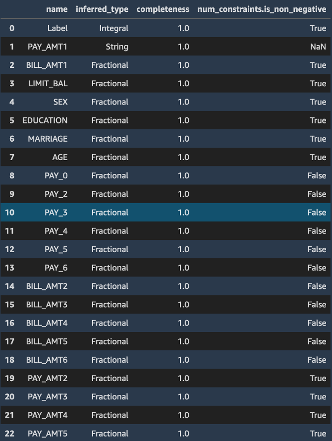
마찬가지로 constraints.json 파일은 비음수 값 및 기능 필드의 데이터 유형과 같이 훈련 데이터 세트가 준수하는 많은 제약 조건으로 구성됩니다.

constraints.json 및 statistics.json의 두 파일을 볼 수 있습니다. 다음에 그 내용을 세부적으로 확인합니다.
위의 코드가 /statistics.json의 json 출력을 pandas 데이터 프레임으로 변환합니다. deequ 라이브러리가 열의 데이터 유형, Null 또는 결측값의 유무 그리고 입력 데이터 스트림의 평균, 최소, 최대, 합계, 표준 편차 및 스케치 파라미터와 같은 통계 파라미터를 추론하는 방법에 유의합니다.
마찬가지로 constraints.json 파일은 비음수 값 및 기능 필드의 데이터 유형과 같이 훈련 데이터 세트가 준수하는 많은 제약 조건으로 구성됩니다.
constraints_df = pd.io.json.json_normalize(baseline_job.suggested_constraints().body_dict["features"])
constraints_df
d. 다음 코드를 실행하여 엔드포인트 모니터링 빈도를 설정합니다.
매일 또는 매시간으로 지정할 수 있습니다. 이 코드는 매시간 빈도를 지정하는데, 매시간 빈도는 많은 데이터를 생성하므로 프로덕션 애플리케이션의 경우 이를 변경할 수도 있습니다. Model Monitor가 탐지한 모든 위반 사항으로 구성된 보고서를 생성합니다.
reports_prefix = '{}/reports'.format(prefix)
s3_report_path = 's3://{}/{}'.format(rawbucket,reports_prefix)
print(s3_report_path)

from sagemaker.model_monitor import CronExpressionGenerator
from time import gmtime, strftime

mon_schedule_name = 'Built-train-deploy-model-monitor-schedule-' + strftime("%Y-%m-%d-%H-%M-%S", gmtime())
my_default_monitor.create_monitoring_schedule(
    monitor_schedule_name=mon_schedule_name,
    endpoint_input=predictor.endpoint,
    output_s3_uri=s3_report_path,
    statistics=my_default_monitor.baseline_statistics(),
    constraints=my_default_monitor.suggested_constraints(),
    schedule_cron_expression=CronExpressionGenerator.hourly(),
    enable_cloudwatch_metrics=True,

)
이 코드가 Amazon CloudWatch Metrics를 활성화하여 Model Monitor에 출력을 CloudWatch로 전송하도록 지시한다는 점에 유의합니다. 이 접근 방식을 사용하면 CloudWatch Alarms를 통해 경보를 트리거하여 데이터 드리프트가 탐지된 시간을 엔지니어 또는 관리자에게 알려줍니다.

9 단계: SageMaker 모델 모니터 성능 테스트
이 단계에서는 일부 샘플 데이터를 사용하여 모델 모니터를 평가합니다. 테스트 페이로드를 있는 그대로 전송하는 대신에 테스트 페이로드의 여러 기능 배포를 수정하여 모델 모니터가 변경 사항을 탐지할 수 있는지 테스트합니다.
모델 모니터 성능을 테스트하려면 다음 단계를 수행하세요.
참고: 자세한 내용은 Amazon SageMaker 설명서의 Amazon SageMaker Model Monitor를 참조하세요.
a. 다음 코드를 실행하여 테스트 데이터를 가져오고 수정된 샘플 데이터를 생성합니다.
COLS = data.columns
test_full = pd.read_csv('test_data.csv', names = ['Label'] +['PAY_AMT1','BILL_AMT1'] + list(COLS[1:])[:11] + list(COLS[1:])[12:17] + list(COLS[1:])[18:]
)
test_full.head()
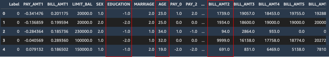
b. 다음 코드를 실행하여 몇 개의 열을 변경합니다. 이전 단계 이미지에서 빨간색으로 표시된 차이에 유의합니다. 레이블 열을 삭제하고 수정된 샘플 테스트 데이터를 저장합니다.
faketestdata = test_full
faketestdata['EDUCATION'] = -faketestdata['EDUCATION'].astype(float)
faketestdata['BILL_AMT2']= (faketestdata['BILL_AMT2']//10).astype(float)
faketestdata['AGE']= (faketestdata['AGE']-10).astype(float)

faketestdata.head()
faketestdata.drop(columns=['Label']).to_csv('test-data-input-cols.csv', index = None, header=None)
c. 다음 코드를 실행하여 수정된 이 데이터 세트로 엔드포인트를 반복 호출합니다.
from threading import Thread

runtime_client = boto3.client('runtime.sagemaker')

# (just repeating code from above for convenience/ able to run this section independently)
def invoke_endpoint(ep_name, file_name, runtime_client):
    with open(file_name, 'r') as f:
        for row in f:
            payload = row.rstrip('\n')
            response = runtime_client.invoke_endpoint(EndpointName=ep_name,
                                          ContentType='text/csv',
                                          Body=payload)
            time.sleep(1)

def invoke_endpoint_forever():
    while True:
        invoke_endpoint(endpoint, 'test-data-input-cols.csv', runtime_client)

thread = Thread(target = invoke_endpoint_forever)
thread.start()
# Note that you need to stop the kernel to stop the invocations
d. 다음 코드를 실행하여 모델 모니터 작업의 상태를 확인합니다.
desc_schedule_result = my_default_monitor.describe_schedule()
print('Schedule status: {}'.format(desc_schedule_result['MonitoringScheduleStatus']))
Schedule status: Scheduled의 출력을 볼 수 있어야 합니다.
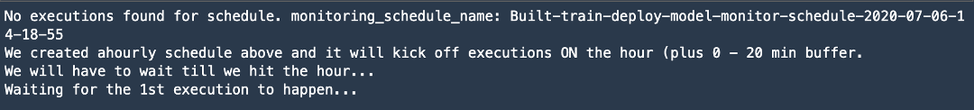
e. 10분마다 모니터링 출력이 생성되었는지 확인하려면 다음 코드를 실행합니다. 첫 번째 작업이 약 20분 동안의 버퍼링이 발생하면서 실행될 수도 있다는 점에 유의합니다.
mon_executions = my_default_monitor.list_executions()
print("We created ahourly schedule above and it will kick off executions ON the hour (plus 0 - 20 min buffer.\nWe will have to wait till we hit the hour...")

while len(mon_executions) == 0:
    print("Waiting for the 1st execution to happen...")
    time.sleep(600)
    mon_executions = my_default_monitor.list_executions()
f. Amazon SageMaker Studio의 왼쪽 도구 모음에서 [엔드포인트(Endpoints)]를 선택합니다. build-train-deploy 엔드포인트를 마우스 오른쪽 버튼으로 클릭하고 [엔드포인트 설명(Describe Endpoint)]을 선택합니다.
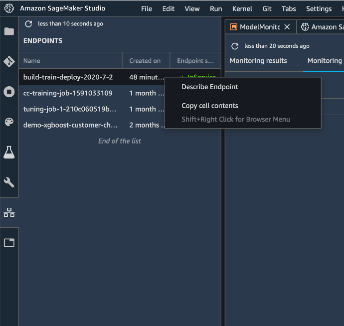
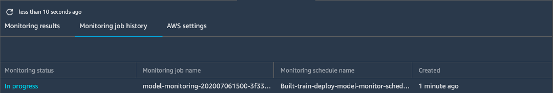
g. [작업 모니터링 기록(Monitoring job history)]을 선택합니다. 모니터링 상태가 [진행 중(In progress)]으로 표시됨에 유의합니다.
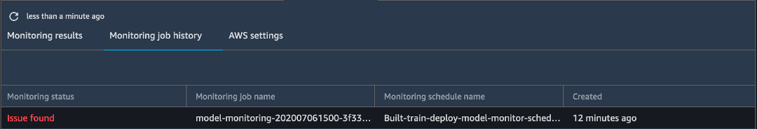
작업이 완료되면 모니터링 상태가 (발견된 문제에 대해) 문제 발견으로 표시됩니다.
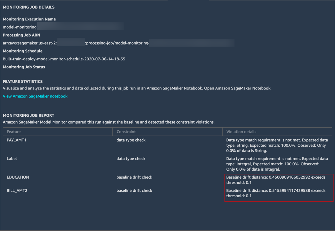
h. 세부 정보를 보려면 문제를 두 번 클릭합니다. Model Monitor가 이전에 수정한 EDUCATION 및 BILL_AMT2 필드에서 대형 기준 드리프트를 탐지한 것을 볼 수 있습니다.
Model Monitor는 또한 두 개의 다른 필드에서도 데이터 유형이 약간 다른 것을 탐지했습니다. 훈련 데이터는 정수 레이블로 구성되며, XGBoost 모델은 확률 점수를 예측합니다. 따라서 모델 모니터가 불일치를 보고했습니다.
i. JupyterLab 노트북에서 다음 셀을 실행하여 모델 모니터의 출력을 확인합니다.
latest_execution = mon_executions[-1] # latest execution's index is -1, second to last is -2 and so on..
time.sleep(60)
latest_execution.wait(logs=False)

print("Latest execution status: {}".format(latest_execution.describe()['ProcessingJobStatus']))
print("Latest execution result: {}".format(latest_execution.describe()['ExitMessage']))

latest_job = latest_execution.describe()
if (latest_job['ProcessingJobStatus'] != 'Completed'):
        print("====STOP==== \n No completed executions to inspect further. Please wait till an execution completes or investigate previously reported failures.")

j. 모델 모니터가 생성한 보고서를 보려면 다음 코드를 실행합니다.
report_uri=latest_execution.output.destination
print('Report Uri: {}'.format(report_uri))
from urllib.parse import urlparse
s3uri = urlparse(report_uri)
report_bucket = s3uri.netloc
report_key = s3uri.path.lstrip('/')
print('Report bucket: {}'.format(report_bucket))
print('Report key: {}'.format(report_key))
s3_client = boto3.Session().client('s3')
result = s3_client.list_objects(Bucket=rawbucket, Prefix=report_key)
report_files = [report_file.get("Key") for report_file in result.get('Contents')]
print("Found Report Files:")
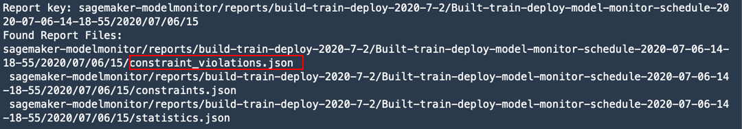
print("\n ".join(report_files))
statistics.json 및 constraints.json 이외에도 constraint_violations.json으로 생성된 새로운 파일을 볼 수 있습니다. 이 파일의 내용은 Amazon SageMaker Studio에서 위에 (단계 g) 표시되었습니다.
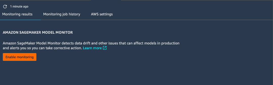
참고: 데이터 캡처를 설정하면 Amazon SageMaker Studio에서 위 코드가 포함된 노트북을 자동으로 생성하여 모니터링 작업을 실행합니다. 노트북에 액세스하려면 엔드포인트를 마우스 오른쪽 버튼으로 클릭하고 [엔드포인트 설명(Describe Endpoint)]을 선택합니다. 모니터링 결과 탭에서 [모니터링 활성화(Enable Monitoring)]를 선택합니다. 이 단계에서는 위에서 작성한 코드가 포함된 Jupyter 노트북이 자동으로 열립니다.
10단계. 정리
이 단계에서는 이번 실습에서 사용한 리소스를 종료합니다.
중요: 비용 절감을 위해 현재 사용 중이지 않은 리소스는 종료하는 것이 좋습니다. 리소스를 종료하지 않으면 계정에 요금이 청구됩니다.
a. 모니터링 일정 삭제: 다음 코드를 복사하여 Jupyter 노트북에 붙여넣은 후에 [실행(Run)]을 선택합니다.
참고: 엔드포인트에 관련되는 모든 모니터링 작업을 삭제하기 전에는 모델 모니터 엔드포인트를 삭제할 수 없습니다.
my_default_monitor.delete_monitoring_schedule()
time.sleep(10) # actually wait for the deletion
b. 엔드포인트 삭제: 다음 코드를 복사하여 Jupyter 노트북에 붙여넣은 다음 [실행(Run)]을 선택합니다.
참고: 먼저 엔드포인트에 관련된 모든 모니터링 작업을 삭제했는지 확인하세요.
sm.delete_endpoint(EndpointName = endpoint_name)모델, 사전 처리한 데이터 세트 등의 모든 훈련 아티팩트를 정리하려면 다음 코드를 복사하여 코드 셀에 붙여넣은 다음 [실행(Run)]을 선택합니다.
참고: ACCOUNT_NUMBER는 실제 계정 번호로 바꿔야 합니다.
%%sh
aws s3 rm --recursive s3://sagemaker-us-east-2-ACCOUNT_NUMBER/sagemaker-modelmonitor/data