Amazon Redshift Engineering’s Advanced Table Design Playbook: Distribution Styles and Distribution Keys

Part 1: Preamble, Prerequisites, and Prioritization
Part 2: Distribution Styles and Distribution Keys (Translated into Japanese)
Part 3: Compound and Interleaved Sort Keys
Part 4: Compression Encodings
Part 5: Table Data Durability

The first table and column properties we discuss in this blog series are table distribution styles (DISTSTYLE) and distribution keys (DISTKEY). This blog installment presents a methodology to guide you through the identification of optimal DISTSTYLEs and DISTKEYs for your unique workload.

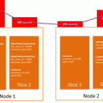
When you load data into a table, Amazon Redshift distributes the rows to each of the compute nodes according to the table’s DISTSTYLE. Within each compute node, the rows are assigned to a cluster slice. Depending on node type, each compute node contains 2, 16, or 32 slices. You can think of a slice like a virtual compute node. During query execution, all slices process the rows that they’ve had assigned in parallel. The primary goal in selecting a table’s DISTSTYLE is to evenly distribute the data throughout the cluster for parallel processing.

When you execute a query, the query optimizer might redistribute or broadcast the intermediate tuples throughout the cluster to facilitate any join or aggregation operations. The secondary goal in selecting a table’s DISTSTYLE is to minimize the cost of data movement necessary for query processing. To achieve minimization, data should be located where it needs to be before the query is executed.

A table might be defined with a DISTSTYLE of EVEN, KEY, or ALL. If you’re unfamiliar with these table properties, you can watch my presentation at the 2016 AWS Santa Clara Summit, where I discussed the basics of distribution starting at the 17-minute mark. I summarize these here:

EVEN will do a round-robin distribution of data.
KEY requires a single column to be defined as a DISTKEY. On ingest, Amazon Redshift hashes each DISTKEY column value, and route hashes to the same slice consistently.
ALL distribution stores a full copy of the table on the first slice of each node.

Which style is most appropriate for your table is determined by several criteria. This post presents a two-phase flow chart that will guide you through questions to ask of your data profile to arrive at the ideal DISTSTYLE and DISTKEY for your scenario.

Phase 1: Identifying Appropriate DISTKEY Columns

Phase 1 seeks to determine if KEY distribution is appropriate. To do so, first determine if the table contains any columns that would appropriately distribute the table data if they were specified as a DISTKEY. If we find that no columns are acceptable DISTKEY columns, then we can eliminate DISTSTYLE KEY as a potential DISTSTYLE option for this table.

o_redshift_table_design_1

Does the column data have a uniformly distributed data profile?

If the hashed column values don’t enable uniform distribution of data to the cluster slices, then you’ll end with both data skew at rest and data skew in flight (during query processing)—which results in a performance hit due to an unevenly parallelized workload. A nonuniformly distributed data profile occurs in scenarios such as these:

Distributing on a column containing a significant percentage of NULL values
Distributing on a column, customer_id, where a minority of your customers are responsible for the majority of your data

You can easily identify columns that contain “heavy hitters” or introduce “hot spots” by using some simple SQL code to review the dataset. In the example following, l_orderkey stands out as a poor option that you can eliminate as a potential DISTKEY column:

root@redshift/dev=# SELECT l_orderkey, COUNT(*) 
FROM lineitem 
GROUP BY 1 
ORDER BY 2 DESC 
LIMIT 100;
 l_orderkey |   count
------------+----------
     [NULL] | 124993010
  260642439 |        80
  240404513 |        80
   56095490 |        72
  348088964 |        72
  466727011 |        72
  438870661 |        72 
...
...

When distributing on a given column, it is desirable to have a nearly consistent number of rows/blocks on each slice. Suppose that you think that you’ve identified a column that should result in uniform distribution but want to confirm this. Here, it’s much more efficient to materialize a single-column temporary table, rather than redistributing the entire table only to find out there was nonuniform distribution:

-- Materialize a single column to check distribution
CREATE TEMP TABLE lineitem_dk_l_partkey DISTKEY (l_partkey) AS 
SELECT l_partkey FROM lineitem;

-- Identify the table OID
root@redshift/tpch=# SELECT 'lineitem_dk_l_partkey'::regclass::oid;
  oid
--------
 240791
(1 row)

Now that the table exists, it’s trivial to review the distribution. In the following query results, we can assess the following characteristics for a given table with a defined DISTKEY:

skew_rows: A ratio of the number of table rows from the slice with the most rows compared to the slice with the fewest table rows. This value defaults to 100.00 if the table doesn’t populate every slice in the cluster. Closer to 1.00 is ideal.
storage_skew: A ratio of the number of blocks consumed by the slice with the most blocks compared to the slice with the fewest blocks. Closer to 1.00 is ideal.
pct_populated: Percentage of slices in the cluster that have at least 1 table row. Closer to 100 is ideal.

SELECT "table" tablename, skew_rows,
  ROUND(CAST(max_blocks_per_slice AS FLOAT) /
  GREATEST(NVL(min_blocks_per_slice,0)::int,1)::FLOAT,5) storage_skew,
  ROUND(CAST(100*dist_slice AS FLOAT) /
  (SELECT COUNT(DISTINCT slice) FROM stv_slices),2) pct_populated
FROM svv_table_info ti
  JOIN (SELECT tbl, MIN(c) min_blocks_per_slice,
          MAX(c) max_blocks_per_slice,
          COUNT(DISTINCT slice) dist_slice
        FROM (SELECT b.tbl, b.slice, COUNT(*) AS c
              FROM STV_BLOCKLIST b
              GROUP BY b.tbl, b.slice)
        WHERE tbl = 240791 GROUP BY tbl) iq ON iq.tbl = ti.table_id;
       tablename       | skew_rows | storage_skew | pct_populated
-----------------------+-----------+--------------+---------------
 lineitem_dk_l_partkey |      1.00 |      1.00259 |           100
(1 row)

Note: A small amount of data skew shouldn’t immediately discourage you from considering an otherwise appropriate distribution key. In many cases, the benefits of collocating large JOIN operations offset the cost of cluster slices processing a slightly uneven workload.

Does the column data have high cardinality?

Cardinality is a relative measure of how many distinct values exist within the column. It’s important to consider cardinality alongside the uniformity of data distribution. In some scenarios, a uniform distribution of data can result in low relative cardinality. Low relative cardinality leads to wasted compute capacity from lack of parallelization. For example, consider a cluster with 576 slices (36x DS2.8XLARGE) and the following table:

CREATE TABLE orders (                                            
  o_orderkey int8 NOT NULL			,
  o_custkey int8 NOT NULL			,
  o_orderstatus char(1) NOT NULL		,
  o_totalprice numeric(12,2) NOT NULL	,
  o_orderdate date NOT NULL DISTKEY ,
  o_orderpriority char(15) NOT NULL	,
  o_clerk char(15) NOT NULL			,
  o_shippriority int4 NOT NULL		,
  o_comment varchar(79) NOT NULL                  
);

Within this table, I retain a billion records representing 12 months of orders. Day to day, I expect that the number of orders remains more or less consistent. This consistency creates a uniformly distributed dataset:

root@redshift/tpch=# SELECT o_orderdate, count(*) 
FROM orders GROUP BY 1 ORDER BY 2 DESC; 
 o_orderdate |  count
-------------+---------
 1993-01-18  | 2651712
 1993-08-29  | 2646252
 1993-12-05  | 2644488
 1993-12-04  | 2642598
...
...
 1993-09-28  | 2593332
 1993-12-12  | 2593164
 1993-11-14  | 2593164
 1993-12-07  | 2592324
(365 rows)

However, the cardinality is relatively low when we compare the 365 distinct values of the o_orderdate DISTKEY column to the 576 cluster slices. If each day’s value were hashed and assigned to an empty slice, this data only populates 63% of the cluster at best. Over 37% of the cluster remains idle during scans against this table. In real-life scenarios, we’ll end up assigning multiple distinct values to already populated slices before we populate each empty slice with at least one value.

-- How many values are assigned to each slice
root@redshift/tpch=# SELECT rows/2592324 assigned_values, COUNT(*) number_of_slices FROM stv_tbl_perm WHERE name='orders' AND slice<6400 
GROUP BY 1 ORDER BY 1;
 assigned_values | number_of_slices
-----------------+------------------
               0 |              307
               1 |              192
               2 |               61
               3 |               13
               4 |                3
(5 rows)

So in this scenario, on one end of the spectrum we have 307 of 576 slices not populated with any day’s worth of data, and on the other end we have 3 slices populated with 4 days’ worth of data. Query execution is limited by the rate at which those 3 slices can process their data. At the same time, over half of the cluster remains idle.

Note: The pct_slices_populated column from the table_inspector.sql query result identifies tables that aren’t fully populating the slices within a cluster.

On the other hand, suppose the o_orderdate DISTKEY column was defined with the timestamp data type and actually stores true order timestamp data (not dates stored as timestamps). In this case, the granularity of the time dimension causes the cardinality of the column to increase from the order of hundreds to the order of millions of distinct values. This approach results in all 576 slices being much more evenly populated.

Note: A timestamp column isn’t usually an appropriate DISTKEY column, because it’s often not joined or aggregated on. However, this case illustrates how relative cardinality can be influenced by data granularity, and the significance it has in resulting in a uniform and complete distribution of table data throughout a cluster.

Do queries perform selective filters on the column?

Even if the DISTKEY column ensures a uniform distribution of data throughout the cluster, suboptimal parallelism can arise if that same column is also used to selectively filter records from the table. To illustrate this, the same orders table with a DISTKEY on o_orderdate is still populated with 1 billion records spanning 365 days of data:

CREATE TABLE orders (                                            
  o_orderkey int8 NOT NULL			,
  o_custkey int8 NOT NULL			,
  o_orderstatus char(1) NOT NULL		,
  o_totalprice numeric(12,2) NOT NULL	,
  o_orderdate date NOT NULL DISTKEY ,
  o_orderpriority char(15) NOT NULL	,
  o_clerk char(15) NOT NULL			,
  o_shippriority int4 NOT NULL		,
  o_comment varchar(79) NOT NULL                  
);

This time, consider the table on a smaller cluster with 80 slices (5x DS2.8XLARGE) instead of 576 slices. With a uniform data distribution and ~4-5x more distinct values than cluster slices, it’s likely that query execution is more evenly parallelized for full table scans of the table. This effect occurs because each slice is more likely to be populated and assigned an equivalent number of records.

However, in many use cases full table scans are uncommon. For example, with time series data it’s more typical for the workload to scan the past 1, 7, or 30 days of data than it is to repeatedly scan the entire table. Let’s assume I have one of these time series data workloads that performs analytics on orders from the last 7 days with SQL patterns, such as the following:

SELECT ... FROM orders 
JOIN ... 
JOIN ... 
WHERE ...
AND o_orderdate between current_date-7 and current_date-1
GROUP BY ...;

With a predicate such as this, we limit the relevant values to just 7 days. All of these days must reside on a maximum of 7 slices within the cluster. Due to consistent hashing, slices that contain one or more of these 7 values contain all of the records for those specific values:

root@redshift/tpch=# SELECT SLICE_NUM(), COUNT(*) FROM orders 
WHERE o_orderdate BETWEEN current_date-7 AND current_date-1 
GROUP BY 1 ORDER BY 1;
 slice_num |  count
-----------+---------
         3 | 2553840
        33 | 2553892
        40 | 2555232
        41 | 2553092
        54 | 2554296
        74 | 2552168
        76 | 2552224
(7 rows)

With the dataset shown above, we have at best 7 slices, each fetching 2.5 million rows to perform further processing. For the scenario with EVEN distribution, we expect 80 slices to fetch ~240,000 records each (((10⁹ records / 365 days) * 7 days) / 80 slices). The important comparison to consider is whether there is in having only 7 slices fetch and process 2.5 million records relative to all 80 slices fetching and processing ~240,000 records each.

If the overhead of having a subset of slices perform the majority of the work is significant, then you want to separate your distribution style from your selective filtering criteria. To do so, choose a different distribution key.

Use the following query to identify how frequently your scans include predicates which filter on the table’s various columns:

SELECT 
    ti."table", ti.diststyle, RTRIM(a.attname) column_name,
    COUNT(DISTINCT s.query ||'-'|| s.segment ||'-'|| s.step) as num_scans,
    COUNT(DISTINCT CASE WHEN TRANSLATE(TRANSLATE(info,')',' '),'(',' ') LIKE ('%'|| a.attname ||'%') THEN s.query ||'-'|| s.segment ||'-'|| s.step END) AS column_filters
FROM stl_explain p
JOIN stl_plan_info i ON ( i.userid=p.userid AND i.query=p.query AND i.nodeid=p.nodeid  )
JOIN stl_scan s ON (s.userid=i.userid AND s.query=i.query AND s.segment=i.segment AND s.step=i.step)
JOIN svv_table_info ti ON ti.table_id=s.tbl
JOIN pg_attribute a ON (a.attrelid=s.tbl AND a.attnum > 0)
WHERE s.tbl IN ([table_id]) 
GROUP BY 1,2,3,a.attnum
ORDER BY attnum;

From this query result, if the potential DISTKEY column is frequently scanned, you can perform further investigation to identify if those filters are extremely selective or not using more complex SQL:

SELECT 
    ti.schemaname||'.'||ti.tablename AS "table", 
    ti.tbl_rows,
    AVG(r.s_rows_pre_filter) avg_s_rows_pre_filter,
    100*ROUND(1::float - AVG(r.s_rows_pre_filter)::float/ti.tbl_rows::float,6) avg_prune_pct,
    AVG(r.s_rows) avg_s_rows,
    100*ROUND(1::float - AVG(r.s_rows)::float/AVG(r.s_rows_pre_filter)::float,6) avg_filter_pct,
    COUNT(DISTINCT i.query) AS num,
    AVG(r.time) AS scan_time,
    MAX(i.query) AS query, TRIM(info) as filter
FROM stl_explain p
JOIN stl_plan_info i ON ( i.userid=p.userid AND i.query=p.query AND i.nodeid=p.nodeid  )
JOIN stl_scan s ON (s.userid=i.userid AND s.query=i.query AND s.segment=i.segment AND s.step=i.step)
JOIN (SELECT table_id,"table" tablename,schema schemaname,tbl_rows,unsorted,sortkey1,sortkey_num,diststyle FROM svv_table_info) ti ON ti.table_id=s.tbl
JOIN (
SELECT query, segment, step, DATEDIFF(s,MIN(starttime),MAX(endtime)) AS time, SUM(rows) s_rows, SUM(rows_pre_filter) s_rows_pre_filter, ROUND(SUM(rows)::float/SUM(rows_pre_filter)::float,6) filter_pct
FROM stl_scan
WHERE userid>1 AND type=2
AND starttime < endtime
GROUP BY 1,2,3
HAVING sum(rows_pre_filter) > 0
) r ON (r.query = i.query and r.segment = i.segment and r.step = i.step)
LEFT JOIN (SELECT attrelid,t.typname FROM pg_attribute a JOIN pg_type t ON t.oid=a.atttypid WHERE attsortkeyord IN (1,-1)) a ON a.attrelid=s.tbl
WHERE s.tbl IN ([table_id])
AND p.info LIKE 'Filter:%' AND p.nodeid > 0
GROUP BY 1,2,10 ORDER BY 1, 9 DESC;

The above SQL describes these items:

tbl_rows: Current number of rows in the table at this moment in time.
avg_s_rows_pre_filter: Number of rows that were actually scanned after the zone maps were leveraged to prune a number of blocks from being fetched.
avg_prune_pct: Percentage of rows that were pruned from the table just by leveraging the zone maps.
avg_s_rows: Number of rows remaining after applying the filter criteria defined in the SQL.
avg_filter_pct: Percentage of rows remaining, relative to avg_s_rows_pre_filter, after a user defined filter has been applied.
num: Number of queries that include this filter criteria.
scan_time: Average number of seconds it takes for the segment which includes that scan to complete.
query: Example query ID for the query that issued these filter criteria.
filter: Detailed filter criteria specified by user.

In the following query results, we can assess the selectivity for a given filter predicate. Your knowledge of the data profile, and how many distinct values exist within a given range constrained by the filter condition, lets you identify whether a filter should be considered selective or not. If you’re not sure of the data profile, you can always construct SQL code from the query results to get a count of distinct values within that range:

table                 | public.orders
tbl_rows              | 22751520
avg_s_rows_pre_filter | 12581124
avg_prune_pct         | 44.7021
avg_s_rows            | 5736106
avg_filter_pct        | 54.407
num                   | 2
scan_time             | 19
query                 | 1721037
filter                | Filter: ((o_orderdate < '1993-08-01'::date) AND (o_orderdate >= '1993-05-01'::date))

SELECT COUNT(DISTINCT o_orderdate) 
FROM public.orders 
WHERE o_orderdate < '1993-08-01' AND o_orderdate >= '1993-05-01';

We’d especially like to avoid columns that have query patterns with these characteristics:

Relative to tbl_rows:
- A low value for avg_s_rows
- A high value for avg_s_rows_pre_filter
A selective filter on the potential DISTKEY column
Limited distinct values within the returned range
High scan_time

If such patterns exist for a column, it’s likely that this column is not a good DISTKEY candidate.

Is the column also a primary compound sortkey column?

Note: Sort keys are discussed in greater detail within Part 3 of this blog series.

As shown in the flow chart, even if we are using the column to selectively filter records (thereby potentially restricting post-scan processing to a portion of the slices), in some circumstances it still makes sense to use the column as the distribution key.

If we selectively filter on the column, we might also be using a sortkey on this column. This approach lets us use the column zone maps effectively on non-necessary slices, to quickly identify the relevant blocks to fetch. Doing this makes selective scanning less expensive by orders of magnitude than a full column scan on each slice. In turn, this lower cost helps to offset the cost of a reduced number of slices processing the bulk of the data after the scan.

You can use the following query to determine the primary sortkey for a table:

SELECT attname FROM pg_attribute 
WHERE attrelid = [table_id] AND attsortkeyord = 1;

Using the SQL code from the last step (used to check avg_s_rows, the number of distinct values in the returned range, and so on), we see the characteristics of a valid DISTKEY option include the following:

Relative to tbl_rows, a low value for avg_s_rows_pre_filter
Relative to avg_s_rows_pre_filter, a similar number for avg_s_rows
Selective filter on the potential DISTKEY column
Numerous distinct values within the returned range
Low or insignificant scan_time

If such patterns exist, it’s likely that this column is a good DISTKEY candidate.

Do the query patterns facilitate MERGE JOINs?

When the following criteria are met, you can use a MERGE JOIN operation, the fastest of the three join operations:

Two tables are sorted (using a compound sort key) and distributed on the same columns.
Both tables are over 80% sorted (svv_table_info.unsorted < 20%)
These tables are joined using the DISTKEY and SORTKEY columns in the JOIN condition.

Because of these restrictive criteria, it’s unusual to encounter a MERGE JOIN operation by chance. Typically, an end user makes explicit design decisions to force this type of JOIN operation, usually because of a requirement for a particular query’s performance. If this JOIN pattern doesn’t exist in your workload, then you won’t benefit from this optimized JOIN operation.

The following query returns the number of statements that scanned your table, scanned another table that was sorted and distributed on the same column, and performed some type of JOIN operation:

SELECT COUNT(*) num_queries FROM stl_query
WHERE query IN (
  SELECT DISTINCT query FROM stl_scan 
  WHERE tbl = [table_id] AND type = 2 AND userid > 1
  INTERSECT
  SELECT DISTINCT query FROM stl_scan 
  WHERE tbl <> [table_id] AND type = 2 AND userid > 1
  AND tbl IN (
    SELECT DISTINCT attrelid FROM pg_attribute 
    WHERE attisdistkey = true AND attsortkeyord > 0
    MINUS
    SELECT DISTINCT attrelid FROM pg_attribute
    WHERE attsortkeyord = -1)
  INTERSECT
  (SELECT DISTINCT query FROM stl_hashjoin WHERE userid > 1
  UNION
  SELECT DISTINCT query FROM stl_nestloop WHERE userid > 1
  UNION
  SELECT DISTINCT query FROM stl_mergejoin WHERE userid > 1)
);

If this query returns any results, you potentially have an opportunity to enable a MERGE JOIN for existing queries without modifying any other tables. If this query returns no results, then you need to proactively tune multiple tables simultaneously to facilitate the performance of a single query.

Note: If a desired MERGE JOIN optimization requires reviewing and modifying multiple tables, you approach the problem in a different fashion than this straightforward approach. This more complex approach goes beyond the scope of this article. If you’re interested in implementing such an optimization, you can check our documentation on the JOIN operations and ask specific questions in the comments at the end of this blog post.

Phase One Recap

Throughout this phase, we answered questions to determine which columns in this table were potentially appropriate DISTKEY columns for our table. At the end of these steps, you might have identified zero to many potential columns for your specific table and dataset. We’ll be keeping these columns (or lack thereof) in mind as we move along to the next phase.

Phase 2: Deciding Distribution Style

Phase 2 dives deeper into the potential distribution styles to determine which is the best choice for your workload. Generally, it’s best to strive for a DISTSTYLE of KEY whenever appropriate. Choose ALL in the scenarios where it makes sense (and KEY doesn’t). Only choose EVEN when neither KEY nor ALL is appropriate.

We’ll work though the following flowchart to assist us with our decision. Because DISTSTYLE is a table property, we run through this analysis table by table, after having completed phase 1 preceding.

o_redshift_table_design_2

Does the table participate in JOINs?

DISTSTYLE ALL is only used to guarantee colocation of JOIN operations, regardless of the columns specified in the JOIN conditions. If the table doesn’t participate in JOIN operations, then DISTSTYLE ALL offers no performance benefits and should be eliminated from consideration.

JOIN operations that benefit from colocation span a robust set of database operations. WHERE clause and JOIN clause join operations (INNER, OUTER, and so on) are obviously included, and so are some not-as-obvious operations and syntax like IN, NOT IN, MINUS/EXCEPT, INTERSECT and EXISTS. When answering whether the table participates in JOINs, consider all of these operations.

This query confirms how many distinct queries have scanned this table and have included one or more JOIN operations at some point in the same query:

SELECT COUNT(*) FROM (
SELECT DISTINCT query FROM stl_scan 
WHERE tbl = [table_id] AND type = 2 AND userid > 1
INTERSECT
(SELECT DISTINCT query FROM stl_hashjoin
UNION
SELECT DISTINCT query FROM stl_nestloop
UNION
SELECT DISTINCT query FROM stl_mergejoin));

If this query returns a count of 0, then the table isn’t participating in any type of JOIN, no matter what operations are in use.

Note: Certain uncommon query patterns can cause the preceding query to return false positives (such as if you have simple scan against your table that is later appended to a result set of a subquery that contains JOINs). If you’re not sure, you can always look at the queries specifically with this code:

SELECT userid, query, starttime, endtime, rtrim(querytxt) qtxt 
FROM stl_query WHERE query IN (
SELECT DISTINCT query FROM stl_scan 
WHERE tbl = [table_id] AND type = 2 AND userid > 1
INTERSECT
(SELECT DISTINCT query FROM stl_hashjoin
UNION
SELECT DISTINCT query FROM stl_nestloop
UNION
SELECT DISTINCT query FROM stl_mergejoin))
ORDER BY starttime;

Does the table contain at least one potential DISTKEY column?

The process detailed in phase 1 helped us to identify a table’s appropriate DISTKEY columns. If no appropriate DISTKEY columns exist, then KEY DISTSTYLE is removed from consideration. If appropriate DISTKEY columns do exist, then EVEN distribution is removed from consideration.

With this simple rule, the decision is never between KEY, EVEN, and ALL—rather it’s between these:

KEY and ALL in cases where at least one valid DISTKEY column exists
EVEN and ALL in cases where no valid DISTKEY columns exist

Can you tolerate additional storage overhead?

To answer whether you can tolerate additional storage overhead, the questions are: How large is the table and how is it currently distributed? You can use the following query to answer these questions:

SELECT table_id, "table", diststyle, size, pct_used 
FROM svv_table_info WHERE table_id = [table_id];

The following example shows how many 1 MB blocks and the percentage of total cluster storage that are currently consumed by duplicate versions of the same orders table with different DISTSTYLEs:

root@redshift/tpch=# SELECT "table", diststyle, size, pct_used
FROM svv_table_info
WHERE "table" LIKE 'orders_diststyle_%';
         table         |    diststyle    | size  | pct_used
-----------------------+-----------------+-------+----------
 orders_diststyle_even | EVEN            |  6740 |   1.1785
 orders_diststyle_key  | KEY(o_orderkey) |  6740 |   1.1785
 orders_diststyle_all  | ALL             | 19983 |   3.4941
(3 rows)

For DISTSTYLE EVEN or KEY, each node receives just a portion of total table data. However, with DISTSTYLE ALL we are storing a complete version of the table on each compute node. For ALL, as we add nodes to a cluster the amount of data per node remains unchanged. Whether this is significant or not depends on your table size, cluster configuration, and storage overhead. If you use a DS2.8XLARGE configuration with 16TB of storage per node, this increase might be a negligible amount of per-node storage. However, if you use a DC1.LARGE configuration with 160GB of storage per node, then the increase in total cluster storage might be an unacceptable increase.

You can multiply the number of nodes by the current size of your KEY or EVEN distributed table to get a rough estimate of the size of the table as DISTSTYLE ALL. This approach should be provide information to determine if ALL results in an unacceptable growth in table storage:

SELECT "table", size, pct_used, 
 CASE diststyle
  WHEN 'ALL' THEN size::TEXT
  ELSE '< ' || size*(SELECT COUNT(DISTINCT node) FROM stv_slices)
 END est_distall_size,
 CASE diststyle
  WHEN 'ALL' THEN pct_used::TEXT
  ELSE '< ' || pct_used*(SELECT COUNT(DISTINCT node) FROM stv_slices)
 END est_distall_pct_used
FROM svv_table_info WHERE table_id = [table_id];

If the estimate is unacceptable, then DISTSTYLE ALL should be removed from consideration.

Do the query patterns tolerate reduced parallelism?

In MPP database systems, performance at scale is achieved by simultaneously processing portions of the complete dataset with several distributed resources. DISTSTYLE ALL means that you’re sacrificing some parallelism, for both read and write operations, to guarantee a colocation of data on each node.

At some point, the benefits of DISTSTYLE ALL tables are offset by the parallelism reduction. At this point, DISTSTYLE ALL is not a valid option. Where that threshold occurs is different for your write operations and your read operations.

Write operations

For a table with KEY or EVEN DISTSTYLE, database write operations are parallelized across each of the slices. This parallelism means that each slice needs to process only a portion of the complete write operation. For ALL distribution, the write operation doesn’t benefit from parallelism because the write needs to be performed in full on every single node to keep the full dataset synchronized on all nodes. This approach significantly reduces performance compared to the same type of write operation performed on a KEY or EVEN distributed table.

If your table is the target of frequent write operations and you find you can’t tolerate the performance hit, that eliminates DISTSTYLE ALL from consideration.

This query identifies how many write operations have modified a table:

SELECT '[table_id]' AS "table_id", 
(SELECT count(*) FROM 
(SELECT DISTINCT query FROM stl_insert WHERE tbl = [table_id]
INTERSECT
SELECT DISTINCT query FROM stl_delete WHERE tbl = [table_id])) AS num_updates,
(SELECT count(*) FROM 
(SELECT DISTINCT query FROM stl_delete WHERE tbl = [table_id]
MINUS
SELECT DISTINCT query FROM stl_insert WHERE tbl = [table_id])) AS num_deletes,
(SELECT COUNT(*) FROM 
(SELECT DISTINCT query FROM stl_insert WHERE tbl = [table_id] 
MINUS 
SELECT distinct query FROM stl_s3client
MINUS
SELECT DISTINCT query FROM stl_delete WHERE tbl = [table_id])) AS num_inserts,
(SELECT COUNT(*) FROM 
(SELECT DISTINCT query FROM stl_insert WHERE tbl = [table_id]
INTERSECT
SELECT distinct query FROM stl_s3client)) as num_copies,
(SELECT COUNT(*) FROM 
(SELECT DISTINCT xid FROM stl_vacuum WHERE table_id = [table_id]
AND status NOT LIKE 'Skipped%')) AS num_vacuum;

If your table is rarely written to, or if you can tolerate the performance hit, then DISTSTYLE ALL is still a valid option.

Read operations

Reads that access DISTSTYLE ALL tables require slices to scan and process the same data multiple times for a single query operation. This approach seeks to improve query performance by avoiding the network I/O overhead of broadcasting or redistributing data to facilitate a join or aggregation. At the same time, it increases the necessary compute and disk I/O due to the excess work being performed over the same data multiple times.

Suppose that you access the table in many ways, sometimes joining, sometimes not. In this case, you’ll need to determine if the benefit of collocating JOINs with DISTSTYLE ALL is significant and desirable or if the cost of reduced parallelism impacts your queries more significantly.

Patterns and trends to avoid

DISTSTYLE ALL tables are most appropriate for smaller, slowly changing dimension tables. As a general set of guidelines, the patterns following typically suggest that DISTSTYLE ALL is a poor option for a given table:

Read operations:
- Scans against large fact tables
- Single table scans that are not participating in JOINs
- Scans against tables with complex aggregations (for example, several windowing aggregates with different partitioning, ordering, and frame clauses)
Write operations:
- A table that is frequently modified with DML statements
- A table that is ingested with massive data loads
- A table that requires frequent maintenance with VACUUM or VACUUM REINDEX operations

If your table is accessed in a way that meets these criteria, then DISTSTYLE ALL is unlikely to be a valid option.

Do the query patterns utilize potential DISTKEY columns in JOIN conditions?

If the table participates in JOIN operations and has appropriate DISTKEY columns, then we need to decide between KEY or ALL distribution styles. Considering only how the table participates in JOIN operations, and no other outside factors, these criteria apply:

ALL distribution is most appropriate when any of these are true:
The table participates in JOINs with multiple column configurations in the JOIN conditiono The most valued JOIN condition doesn’t use an appropriate DISTKEY columno The table participates in equally valued JOINs, with conditions on differing columns

KEY distribution is most appropriate when important JOIN conditions consistently include one potential DISTKEY column

Determining the best DISTKEY column

If you’ve determined that DISTSTYLE KEY is best for your table, the next step is to determine which column serves as the ideal DISTKEY column. Of the columns you’ve flagged as appropriate potential DISTKEY columns in phase 1, you’ll want to identify which has the largest impact on your particular workload.

For tables with only a single candidate column, or for workloads that only use one of the candidate columns in JOINs, the choice is obvious. For workloads with mixed JOIN conditions against the same table, the most optimal column is determined based on your business requirements.

For example, common scenarios to encounter and questions to ask yourself about how you want to distribute are the following:

My transformation SQL code and reporting workload benefit from different columns. Do I want to facilitate my transformation job or reporting performance?
My dashboard queries and structured reports leverage different JOIN conditions. Do I value interactive query end user experience over business-critical report SLAs?
Should I distribute on column_A that occurs in a JOIN condition thousands of times daily for less important analytics, or on column_B that is referenced only tens of times daily for more important analytics? Would I rather improve a 5 second query to 2 seconds 1,000 times per day, or improve a 60-minute query to 24 minutes twice per day?

Your business requirements and where you place value answer these questions, so there is no simple way to offer guidance that covers all scenarios. If you have a scenario with mixed JOIN conditions and no real winner in value, you can always test multiple distribution key options and measure what works best for you. Or you can materialize multiple copies of the table distributed on differing columns and route queries to disparate tables based on query requirements. If you end up attempting the latter approach, pgbouncer-rr is a great utility to simplify the routing of queries for your end users.

Next Steps

Choosing optimal DISTSTYLE and DISTKEY options for your table ensures that your data is distributed evenly for parallel processing, and that data redistribution during query execution is minimal—which ensures your complex analytical workloads perform well over multipetabyte datasets.

By following the process detailed preceding, you can identify the ideal DISTSTYLE and DISTKEY for your specific tables. The final step is to simply rebuild the tables to apply these optimizations. This rebuild can be performed at any time. However, if you intend to continue reading through parts 3, 4, and 5 of the Advanced Table Design Playbook, you might want to wait until the end before you issue the table rebuilds. Otherwise, you might find yourself rebuilding these tables multiple times to implement optimizations identified in later installments.

In Part 3 of our table design playbook, I’ll describe how to use table properties related to table sorting styles and sort keys for another significant performance gain.