AWS Big Data Blog
How Annalect built an event log data analytics solution using Amazon Redshift
Ingesting and analyzing event log data into a data warehouse in near real-time is challenging. Data ingest must be fast and efficient. The data warehouse must be able to scale quickly to handle incoming data volumes. Storing massive amounts of historical data in the data warehouse for infrequent access is prohibitively expensive. If you store infrequently accessed data outside the data warehouse, loading time is unacceptable.
At Annalect, we found a way to overcome these challenges. In this article, we discuss how we built a solution on AWS to manage, enhance, and analyze event log data from our ad technology partners. We use Amazon S3 for storage, Amazon EC2 and AWS Batch for compute, AWS Glue Data Catalog, and Amazon Redshift and Amazon Redshift Spectrum for analytics. This scalable, on-demand architecture has proven to be a high-performance solution for our analytics users and is very cost-effective.
Architecture overview
In mid-2016, we were using Amazon Redshift with local tables to provide SQL access to event-level ad tech datasets for analysts and modelers to improve ad buying strategies. We retained up to six months of historical data for select data sources; this represented about 230 billion events. By early 2017, the same data footprint grew to over 385 billion events, and we increased our Amazon Redshift capacity to keep pace. As we looked forward, we wanted to support more data, both in terms of history and data source coverage. At the same time, we wanted to maintain or improve query performance, ideally without increasing costs.
Because we were already using Amazon Redshift as our data warehouse, we looked at Redshift Spectrum. Redshift Spectrum is a feature of Amazon Redshift that queries data stored in Amazon S3. It uses the same SQL capabilities as Amazon Redshift, without the need to load the data into Amazon Redshift tables stored on disks within an Amazon Redshift cluster.
With Redshift Spectrum, a table’s storage is separate from a cluster’s compute resources, which enables each to scale independently of the other. We can keep large data tables in S3 instead of local Amazon Redshift storage, which reduces the size of our Amazon Redshift clusters and lowers costs. Queries that use external Redshift Spectrum tables use Redshift Spectrum compute resources (separate from the Amazon Redshift cluster) to scan the data in S3. Queries are billed by AWS at a metered rate based on the amount of data scanned. For query efficiency, we convert the data stored in S3 into Parquet files using AWS Batch.
The result is an efficient, mostly serverless analytics environment where the data is always available to query with Redshift Spectrum. Although we manage some always-on Amazon Redshift clusters, we think of this as “mostly serverless.” This is because the cluster footprint is very small relative to the serverless compute power we use through Redshift Spectrum for analysis and through AWS Batch for data preparation.
The Amazon Redshift clusters are dedicated to performing analytics for our analysts, rather than having a portion of their time dedicated to load jobs. This is because no time is spent copying data into local tables in the Amazon Redshift clusters and because we do the data preparation work outside of Amazon Redshift.
With the evolution to Redshift Spectrum and storing table data in S3, by early 2018 we increased the amount of data that we deliver to analysts by an order of magnitude. At the same time, we kept our costs at the same level as 2017. Using Redshift Spectrum is a great cost saving to us. We now have up to 36 months of historical data available for many more data sources, representing trillions of events.
Our data management infrastructure, the Enhanced Event-Level Data Environment (EELDE), is structured as shown following.
The EELDE provides four primary functions:
- Data ingest
- Data transformation
- Compute-intensive enrichment
- Analyst ad hoc query environment
These four functions are described following in more detail.
Data ingest
We architected our ingest system to ensure smooth and rapid downstream data availability. We took into account the inherent inconsistencies of vendor data feeds, both in the contents of the feeds themselves and in different vendors’ data push conventions. We also took into account the large volume of data files that data vendors might deliver at a given time. The diagram following shows our data ingest process.

We set up two storage areas in Amazon S3 to initially hold data from our vendors. The Landing Zone serves as a repository for long-term storage of historical, unaltered raw log files. Log files that are pulled by us directly from vendors are stored immediately in the Landing Zone. The Datafeeds storage serves as a transient place for log files that are pushed out by the vendors. We curate and arrange the data files delivered into the Datafeeds storage by vendors as we pull them into the Landing Zone.
The pull processes are executed in the EELDE’s Job Execution Layer, which is autoscaling and can handle many data files in parallel. This ensures that data processing and availability are not delayed by sudden spikes in data volume. Some spikes might occur from the need to backfill a large dataset from a new vendor. Others might occur when a vendor delivers a large volume of logs accumulated after a delay on their side.
Whether the vendor logs are pushed or pulled, we monitor the Landing Zone. We send alerts when we detect changes in file formats or gaps in data that might have an impact on downstream analysis. We found that this architecture and process gives us the control, flexibility, and agility that we need to respond rapidly to any volume of data and any changes in the data.
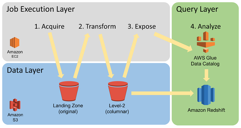
Data transformation
The EELDE can process, enhance, and analyze large volumes of event data in a compute-efficient and cost-efficient manner. An important part of this ability is the initial transformation of files in the Landing Zone. The EELDE’s Job Execution Layer uses AWS Batch to parallelize the compute-intensive data transformation from the original source data. This data is typically in comma-separated value (CSV) or JSON format. AWS Batch parallelizes it into a columnar, compressed storage format, Apache Parquet. In the diagrams, you can see the Parquet storage location labeled as the “Level 2 (columnar)” bucket.
For our Parquet transformation jobs, we have had a good experience running many containers with local-mode Apache Spark using AWS Batch. The goal for us is supporting a high throughput of file transformations where each file’s size is in the range of a few megabytes to a few gigabytes. A given Parquet transformation might take anywhere from a few seconds to 30 minutes.
The resource isolation and job management provided by AWS Batch makes running hundreds of independent data transformation jobs straightforward. At the same time, it removes some of the challenges of running many tasks simultaneously within Amazon EMR. In contrast, to transform larger datasets, the parallel compute per job that EMR can provide is attractive.
The diagram following shows data transformation and cataloging.

We partition the large Parquet-backed event data tables by date. Date partitioning is strategically implemented to optimize both query cost and query performance by providing an efficient path to the required data for a given analytics process. After the files are converted to Parquet, they are exposed as table partitions in the AWS Glue Data Catalog. Although the data storage format has been transformed, the data still retains all of its original fields, which is important for supporting ad hoc analyses.
Once the Parquet conversion and AWS Glue Data Catalog management processes have run, the data is accessible through SQL queries using Redshift Spectrum. Redshift Spectrum uses the AWS Glue Data Catalog to reference external tables stored in S3 so that you can query them through the Amazon Redshift cluster. Using a columnar format like Parquet increases the speed and cost efficiency of performing queries with Redshift Spectrum.
Compute-intensive enrichment
Before analytics work, the Job Execution Layer might also run other compute intensive data transformations to enhance the logs so that they can support more advanced types of analysis. Event-level log combination and event attribute augmentation are two examples.
Although these enrichment tasks might have different compute requirements, they can all use Redshift Spectrum to gather relevant datasets, which are then processed in the Job Execution Layer. The results are made available again through Redshift Spectrum. This enables complex enrichment of large datasets in acceptable timeframes and at a low cost.
Analyst ad hoc query environment
Our environment provides analysts with a data landscape and SQL query environment for mission-critical analytics. The data is organized within the EELDE into separate external schemas by ad tech vendor and system seat or account. Our agency-based analysts and data scientists are granted access to specific schemas according to project needs.
By having access to various datasets within a single platform, analysts can gain unique insights that are not possible by analyzing data in separate silos. They can create new datasets from a combination of source vendors for use during specific analytic projects while respecting data separation requirements. Doing this helps support use cases such as predictive modeling, channel planning, and multisource attribution.
Best practices to keep costs low
Along the way, we have developed some best practices for Redshift Spectrum:
- Use compressed columnar format. We use Apache Parquet for our large event-level tables. Doing this reduces query run time, data scan costs, and storage costs. Our large tables typically have 40–200 columns, yet most of our queries use only 4–8 columns at a time. Using Parquet commonly lowers the scan cost by over 90 percent compared to noncolumnar alternatives.
- Partition tables. We partition our large event level tables by date, and we train users to use the partition column in WHERE clauses. Doing this provides cost savings proportional to the portion of dates used by the queries. For example, suppose that we expose six months of data and a query looks at only one month. In this case, the cost for that query is reduced by five-sixths by using the appropriate WHERE clause.
- Actively manage table partitions. Although we have up to 36 months of historical data available as Parquet files, by default we expose only the most recent 6 months of data as external table partitions. This practice reduces the cost of queries when users fail to filter on the partition column. On request, we temporarily add older date partitions to the necessary tables to support queries that need more than 6 months of data. In this way, we support longer timeframes when needed. At the same time, we usually maintain a lower cost limit by not exposing more data than is commonly necessary.
- Move external tables into Amazon Redshift when necessary. When a large number of queries repeatedly hit the same external table, we often create a temporary local table in Amazon Redshift to query against. Depending on the number of queries and their scope, it can be helpful to load the data into a local Amazon Redshift table with the appropriate distribution key and sort keys. This practice helps eliminate the repeated Redshift Spectrum scan costs.
- Use spectrum_scan_size_mb WLM rules. Most of our users and jobs operate with an effective Redshift Spectrum data scan limit of 1 terabyte by setting a spectrum_scan_size_mb WLM rule on the default WLM queue. For a single analysis or modeling query, this limit rarely needs to be exceeded.
- Add clusters to increase concurrency when needed. Multiple Amazon Redshift clusters have access to the same external tables in S3. If we have a lot of users running queries at the same time against external tables, we might choose to add more clusters. Redshift Spectrum and the management tools we have created for our environment make this an easy task.
- Use short-lived Amazon Redshift clusters. For some scheduled production jobs, we use short-lived Amazon Redshift clusters with the necessary data made available through external schemas. Redshift Spectrum allows us to avoid lengthy data load times, so it is practical to launch a Amazon Redshift cluster for a couple of hours of work and then terminate it every day. Doing this can save 80–90 percent compared to having an always-on cluster for a project. It also avoids contention with other query activity, because the short-lived cluster is dedicated to the project.
Summary
By establishing a data warehouse strategy using Amazon S3 for storage and Redshift Spectrum for analytics, we increased the size of the datasets we support by over an order of magnitude. In addition, we improved our ability to ingest large volumes of data quickly, and maintained fast performance without increasing our costs. Our analysts and modelers can now perform deeper analytics to improve ad buying strategies and results.
Additional Reading
If you found this post useful, be sure to check out Using Amazon Redshift Spectrum, Amazon Athena, and AWS Glue with Node.js in Production and How I built a data warehouse using Amazon Redshift and AWS services in record time.
About the Author
 Eric Kamm is a senior engineer and architect at Annalect. He has been creating and managing large-scale ETL workflows and providing data and compute environments for teams of analysts and modelers for over twenty years. He enjoys working with cloud technologies because they can accelerate project planning and implementation while increasing reliability and operational efficiency.