AWS Quantum Technologies Blog
Exploring Quantum Measurements, Observables and Operators: Practical insights with Amazon Braket
Introduction
In this post, we explore the mathematical foundations and practical implementations of quantum measurement techniques using Amazon Braket. We examine this subject through multiple perspectives: action of gates as basis transformation, projection as inner product, projector formalism, and observable formalism. A key insight that we’ll develop is understanding basis transformations as tools for converting phase information to amplitude information – a concept central to many quantum algorithms.
This post aims to provide both intuitive understanding and implementation ideas for those looking to deepen their understanding of quantum measurement techniques.
Superposition and Measurement in Arbitrary Basis
A general one-qubit state can be written as a superposition in the computational basis {|0⟩, |1⟩}: |ψ⟩ = α₀|0⟩ + α₁|1⟩, where α₀ and α₁ are complex probability amplitudes satisfying |α₀|² + |α₁|² = 1. These amplitudes quantify the projection (or overlap) of the state onto the basis vectors.
Quantum measurement determines the degree of projection of the state onto the measurement basis. Now consider measuring this state in a different orthonormal basis {|u₀⟩, |u₁⟩}. To represent the state in this arbitrary basis as |ψ⟩ = β₀|u₀⟩ + β₁|u₁⟩, we need to find coefficients β₀ and β₁.
Consider the unitary matrix U with {|u₀⟩, |u₁⟩} as columns: U = [|u₀⟩ |u₁⟩]
To find β₀ and β₁ in |ψ⟩ = β₀|u₀⟩ + β₁|u₁⟩, we express the new basis vectors in terms of the computational basis:
Note that U|0⟩ = |u₀⟩ and U|1⟩ = |u₁⟩.
|ψ⟩ = β₀U|0⟩ + β₁U|1⟩ = U(β₀|0⟩ + β₁|1⟩)
Since U is unitary, applying U† to both sides yields: U†|ψ⟩ = β₀|0⟩ + β₁|1⟩
The coefficients β₀ and β₁ are the projections of U†|ψ⟩ onto the computational basis states. Therefore, measuring U†|ψ⟩ in the computational basis gives identical results to measuring the original state |ψ⟩ in the {|u₀⟩, |u₁⟩} basis.
This idea naturally generalizes to n-qubit system.
An n-qubit system lives in N = 2n dimensional Hilbert space (with 2n basis vectors). In the computational basis, these 2n basis are denoted by the binary strings of numerals from 0 to 2n -1: |00…0⟩, |00…1⟩……|11…1⟩.
A general state |ψ⟩ can be expressed in the computational basis as
|ψ⟩ = α0 |00…0⟩ + α1 |00…1⟩ + …. + αN-1 |11…1⟩ or simply ∑k αk |k⟩ where 0 <= k <= 2n -1 and ∑ |αk|² = 1 (normalization condition).
Suppose we now want to measure this state in any other arbitrary orthonormal basis {|u0⟩, |u₁⟩…|uk⟩, …, |uN-1⟩}. When we measure |ψ⟩ in this basis, we are, in effect, asking: “What is the probability of finding the system in state |uk⟩?”
The state |ψ⟩ can then be expressed in this basis as
|ψ⟩ = β0 |u0⟩ + β1 |u1⟩ + …. + βN-1 |uN-1⟩ where βₖ = ⟨uₖ|ψ⟩ is the amplitude of the state projected onto basis |uₖ⟩.
As before, if U is a unitary matrix whose columns are = {|u₀⟩ |u₁⟩ … |uN-1⟩},
U†|ψ⟩ = ∑k βₖ |uk⟩ = β0 |00…0⟩ + β1 |00…1⟩ + …. + βN-1 |11…1⟩
Measuring |ψ⟩ in the basis {|uk⟩} is equivalent to applying U† to the state and measuring in the computational basis.
Conversely, let V be any unitary operator (quantum gate). Then applying gate V to state |ψ⟩ and measuring the result V|ψ⟩ in the computational basis is equivalent to measuring the original state |ψ⟩ in the basis formed by the columns of V†.
This is an important principle of quantum measurement. Physical devices permit measurement in Z basis (the computational basis). The notion of measurement in a different basis is then achieved by an equivalent unitary transformation.
Let us now view this through an example. In the following diagram (figure 1), a single qubit quantum state |ψ⟩ is represented in Real 2D vector space (with probability amplitudes as real numbers)
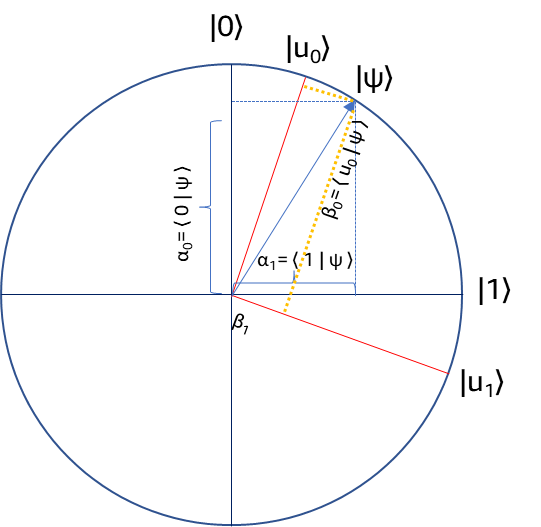
Figure 1: Representation of a state in different basis on real 2D plane. |0⟩ and |1⟩ represent the computational basis while |u0⟩ and |u1⟩ represent any arbitrary basis. |ψ⟩ represents a single qubit state. The projections of the state on each basis vectors are inner products of the state with the respective basis vectors.
Consider a state vector |ψ⟩ oriented at π/6 (30°) from |0⟩.
Then, the state can be represented in the computational basis as:
|ψ⟩ = cos(π/6)|0⟩ + sin(π/6)|1⟩ = √3/2|0⟩ + 1/2|1⟩
In the computational basis {|0⟩, |1⟩}:
- Probability of measuring |0⟩: |cos(π/6)|² = 3/4 = 75%
- Probability of measuring |1⟩: |sin(π/6)|² = 1/4 = 25%
Now consider measuring this same state in an arbitrary orthonormal basis {|u₀⟩, |u₁⟩} that is at an angle of π/8 (22.5°) from the computational basis {|0⟩, |1⟩}:
|u₀⟩ = cos(π/8)|0⟩ + sin(π/8)|1⟩
|u₁⟩ = -sin(π/8)|0⟩ + cos(π/8)|1⟩
The measurement outcomes will depend on the projection of state |ψ⟩ onto these basis vectors.
Analytically, we can see that:
|ψ⟩ = cos(π/24)|u₀⟩ + sin(π/24)|u₁⟩
In the arbitrary orthonormal basis {|u₀⟩, |u₁⟩},
- Probability of measuring |u₀⟩: |cos(π/24)|² ≈ 0.983 = 98.3%
- Probability of measuring |u₁⟩: |sin(π/24)|² ≈ 0.017 = 1.7%
Note on Bloch Sphere Representation:
On the Bloch sphere, angular parameters are twice the physical angles in the state space. A rotation by an angle θ in state space corresponds to a rotation by 2θ on the Bloch sphere. This relates to the SU(2) group being a double cover of SO(3) (see references for details).
Let us now see this using Amazon Braket.
As shown in the code below, first, we create an instance of LocalSimulator and a Circuit. Amazon Braket initializes qubits to |0⟩ (oriented along the Z axis of Bloch Sphere). We then rotate the state by an angle 30 degrees (π/6) along the Y axis. Note that a physical rotation of (π/6) corresponds to a rotation of (π/3) on Bloch Sphere. The qubit state stays in XZ plane of Bloch Sphere. This corresponds to the representation in Figure 1.
We create two vectors u_0 and u_1 that denote the measurement basis of our interest. It can be easily seen that these are orthogonal (the inner product is zero). We then create a matrix with these two vectors as columns. For higher dimensions, the same pattern applies. We then take the adjoint of this matrix – since our scenario is with real values, transpose of this matrix is taken (which will be the same as adjoint). The resultant matrix will also be unitary. This unitary operator is then applied to the state (Circuit object) using “Circuit.unitary” method. We then measure the state in the computational basis. Note that the measurement method in Amazon Braket is by default on the computational basis.
Code: Measuring in an arbitrary basis
import numpy as np
from braket.circuits import Circuit
from braket.devices import LocalSimulator

device = LocalSimulator()
circuit = Circuit()

# qubits in Braket are initialized to "0" and aligned with Z axis. Rotate the qubit about the Y axis by an angle (in radians). Though we set the orientation of the qubit and very much know the exact state, we will pretend that we do not know this and will determine this through measurement operations (the purpose of this example).

state_angle = np.pi / 3
circuit.ry(0, state_angle)

# Define a Basis Vector that is at an orientation of pi/8 from computational basis 0
u_0 = np.array([[np.cos(np.pi/8)], [np.sin(np.pi/8)]])

# Define a Basis Vector that is at an orientation of pi/8 from computational basis 1. This is orthonormal to u_0
u_1 = np.array([[-np.sin(np.pi/8)], [np.cos(np.pi/8)]])

# Form a matrix that has the basis of measurement as its columns
matrix_formed_from_basis_vectors = np.hstack((u_0, u_1))

#The unitary gate will then be the adjoint of the matrix formed above
#For real matrix, adjoint is same as transpose.
basis_rotation_gate = matrix_formed_from_basis_vectors.T

# Apply this unitary gate to the circuit - in effect, this is a coordinate rotation
circuit.unitary(matrix=basis_rotation_gate, targets=[0])
circuit.probability(target=0)

task = device.run(circuit, shots=1000)
taskResult = task.result()

measurement_probabilties = taskResult.values[0]
counts = taskResult.measurement_counts

print("Probability : ", measurement_probabilties)
print("Counts : ", counts)
Running this code will yield a result similar to this(note that you may get a different number, but it will be close to and tend towards this):
Probability :  [0.983 0.017]
Counts :  Counter({'0': 983, '1': 17})
The result matches with the values derived analytically before.
Why measure in a different basis at all?
Different measurement bases reveal complementary aspects of quantum states. This complementarity arises from the probabilistic nature of quantum measurement: we observe outcomes with specific probabilities via the Born rule, not the underlying complex amplitudes directly.
Consider a general state |ψ⟩ = α|0⟩ + β|1⟩ where α and β are complex numbers. Measurement in the computational basis reveals |α|² and |β|² (the probabilities of outcomes |0⟩ and |1⟩), but not the relative phase between α and β. This phase information remains encoded in the quantum state and is inaccessible through measurements in that particular basis. States differing only in relative phase yield identical measurement statistics in that basis, despite being distinct quantum states.
Example: Accessing Hidden Phase Information
Consider |+⟩ = (|0⟩ + |1⟩)/ √2 and |−⟩ = (|0⟩ − |1⟩)/ √2 . These states differ only in the relative phase between their |0⟩ and |1⟩ components. Notably, despite both being equal superpositions, |+⟩ and |−⟩ are orthogonal states — as maximally distinguishable from each other as |0⟩ and |1⟩ are.
In computational basis measurements, both states yield 50% |0⟩ and 50% |1⟩. The ± phase relationship is not observable. However, in the {|+⟩, |−⟩} basis, |+⟩ always yields |+⟩ and |−⟩ always yields |−⟩ (both with probability = 1). The phase information becomes directly observable.
This illustrates quantum measurement complementarity: complete characterization of a quantum state requires measurements in multiple incompatible bases—bases whose measurement operators do not commute, preventing simultaneous precise measurement. Each measurement basis accesses specific quantum information while rendering other aspects unobservable.
How does a change of basis uncover aspects of quantum information?
Let us go back to the measurement postulate. The probabilities of outcome depend on the projection of the quantum state on the basis states (vectors or subspaces). This can be better visualized in 1 qubit case on a Bloch sphere. An arbitrary state is a point on the Bloch sphere and the projection of that state on the Z axis determines the probability of that state yielding |0⟩ or |1⟩ state upon measurement. Probabilities of states that all lie on the same latitude have the same value. Different points on the Bloch sphere at the same latitude differ from each other only in relative phase.
When we measure the state from a different basis, we are enquiring about the projection of the same state vector on a vector or direction that is different from the computational basis. The states that differ only in phase with respect to the computational basis (and have the same projections on Z direction) cast different projections on measurement basis / axis that is different from the computational basis.
As an analogy, take two cities in a globe that are at the same latitude. They will have the same projection along the north-south axis, but if we reorient and hinge the globe on to equatorial axis, these same cities will cast different projections along this new axis.
The crucial insight is that what appears as “phase” in the computational basis, manifests itself as “amplitude” in a different basis. Since amplitudes determine the measurement outcomes, basis transformation can be viewed as the mechanism to enable this phase to amplitude change.
This is the reason Hadamard transform plays such a critical role in quantum algorithms. As we saw from the previous section, any Unitary transform (such as Hadamard) can be viewed and interpreted as a basis transformation (coordinate rotation). Hadamard transform changes the computational basis {|0⟩, |1⟩} perspective to |+⟩ and |-⟩ perspective. Information that is encoded in phase (in algorithms such as Simon’s, Shor’s and any phase kickback dependent procedure) use the basis transformation approach to uncover the pattern in the quantum information.
We can draw a couple of key points from this analysis:
- The choice of basis of measurement gives us unique perspectives that may not be available from another basis; and we cannot get all perspectives simultaneously. A greater certainty of measurement in one basis set may a greater uncertainty in the corresponding basis from another set.
- We can interpret the operation of a Unitary matrix on a state in two ways – either as Unitary matrix changing the state of the system, or alternatively, as basis transformation which enables measurement (or viewing angle) on the qubit from a different coordinate system
Projector formulation for measuring a state in an arbitrary basis
In quantum mechanics, physical measurements are described by Observables. This measurement is about determining how much of a quantum state “projects onto” each basis vector. This geometric intuition of projection is captured using the notion of projectors, which serve as the elementary building blocks for understanding measurements using Observables
We saw that probability that a state |ψ⟩, when measured in an arbitrary basis {|u0⟩, |u₁⟩…|uk⟩, …, |uN-1⟩}, is seen in state |uk⟩ is |⟨uₖ|ψ⟩|² = ⟨uk|ψ⟩⟨uk|ψ⟩* = ⟨uk|ψ⟩⟨ψ|uk⟩ = ⟨ψ|uk⟩⟨uk|ψ⟩
The outer product expression |uk⟩⟨uk| is called the projector for the basis state |uk⟩. Let us denote it by Pk. Therefore, the probability of obtaining an outcome state |uk⟩ when |ψ⟩ is measured in the basis {|u0⟩, |u₁⟩…|uk⟩, …, |uN-1⟩} is ⟨ψ|Pk|ψ⟩.
The projector Pₖ can be understood as an operation that extracts the component of |ψ⟩ that lies along direction |uₖ⟩.
Pk|ψ⟩ = |uk⟩⟨uk|ψ⟩
⟨uk|ψ⟩ is the complex amplitude quantifying the “overlap” between |ψ⟩ and |uk⟩, and Pk|ψ⟩ scales |uk⟩ by this amplitude, yielding the component of |ψ⟩ that lies along |uk⟩.
Projectors can be viewed as the fundamental building blocks of quantum observables. Action of a projector represents the most basic type of measurement in quantum mechanics. A Projector P asks the elementary (“yes”/”no”) question: “Is the system in a state defined by the projector ?”. We will get the answer “Yes” with a probability ⟨ψ|P|ψ⟩.
Projectors are Hermitian operators with eigenvalues 0 and 1. They preserve components in their target subspace (eigenvalue 1) while removing orthogonal components (eigenvalue 0).
From Projectors to Observables
Projectors answer binary “yes/no” questions about quantum states within a specific direction or subspace. An Observable extends this concept by assigning numerical values to different measurement outcomes.
An Observable is essentially a construct that measures a quantum state in the basis defined by its eigenvectors. Each observable implicitly defines a measurement basis – its eigenbasis – determining the “reference frame” in which the quantum state is observed.
Mathematically, an observable is a weighted sum of orthogonal projectors:
A = λ0P0 + λ1P1 + … + λₙ-1Pn-1 (Spectral Decomposition of an observable)
where each λᵢ is a real eigenvalue and Pᵢ is the projector onto the corresponding eigenspace.
When we measure an observable A in a state |ψ⟩, each measurement yields exactly one of the eigenvalues λᵢ. The probability of obtaining λᵢ is ⟨ψ|Pᵢ|ψ⟩. Upon measurement, the state “collapses” to a new state Pᵢ|ψ⟩/√ψ|Pᵢ|ψ . The denominator is the normalization factor to account for the unit normal requirement of a quantum state.
Put differently, an observable provides a measurement model that uses its eigenvectors as the measurement basis and produces eigenvalues as measurement outcomes. For example, measuring with Pauli X observable is equivalent to measuring in |+⟩ and |-⟩ basis and measuring with Pauli Z is nothing but measuring in |0⟩ and |1⟩ basis (|+⟩ and |-⟩ are the eigenvectors of X and |0⟩ and |1⟩ are the eigenvectors of Z). The measurement outcome follows a probability distribution determined by the quantum state’s projection onto each eigenspace.
Each experimental “shot” on a device (simulator or real quantum hardware) represents a single measurement instance, causing the quantum state to collapse to one of the eigenspaces while yielding the corresponding eigenvalue as the measurement result. The expectation value of a measurement is then the weighted sum of all the measurement shots. It is pertinent to reiterate that each measurement shot always yields one of the eigenvalues. We never see the “expectation value” during any specific observation. This is a statistical average post computed from results of individual measurement.
A projector operator may be viewed as the most elementary observable that has just one eigenvalue and its value is 1. In other words, it is the Observable that just has one component in its spectral decomposition.
An Observable, in general, gives the expectation value – this is the statistical average of the eigenvalues we assign to each of the measurement basis (the eigenstate – note that when we use an observable, we are implicitly measuring the state in the eigenvector(eigenstate) of the observable). A measurement using an elementary projector (as Observable), will give probability directly – this is because the eigenvalue of the projector is 1 and this unit value does not affect the statistics of measurement.
Observable as a sum of Pauli Terms
In principle, any Hermitian operator A with orthonormal eigenvectors can serve as a quantum observable, where measurements project onto these eigenstates with corresponding eigenvalues λᵢ. The observable A = Σᵢ λᵢ|uᵢ⟩⟨uᵢ| represents the complete measurement in this custom basis. Most quantum hardware can only perform measurements in a single, fixed computational basis—the Z-basis (|0⟩, |1⟩).
Quantum computing frameworks solve this through a systematic decomposition process:
Any single-qubit Hermitian operator A can be uniquely decomposed as: A = a₀I + a₁X + a₂Y + a₃Z. Here, aᵢ are real number coefficients and X, Y, and Z are the three Pauli matrices (Observables) along with Identity matrix I.

Pauli measurements use Pauli matrices as observables. When we use a custom Hermitian as an Observable, Amazon Braket decomposes it into this linear combination of Pauli observables. Each Pauli operator can then be reinterpreted in terms of Pauli-Z computational basis measurements through appropriate basis rotations, completing the translation from arbitrary measurements to physically implementable operations.
Pauli X measurement is implemented by applying Hadamard gate (H) before a Z basis measurement; Pauli Y measurement is implemented by first applying S† (phase gate) and then Hadamard gate followed by the Z basis measurement.

Measuring in an arbitrary basis using Observable in Amazon Braket
The following code illustrates using a projector to measure the state of a system in the basis {|u0⟩, |u₁⟩) as in previous example.
First, we define a method to create a projector, given a basis vector. A projector in its most basic form is an outer product of the basis vector with itself. This projector gives the probability that the state is seen in the basis defined by the vector used for creating it.
We define the two basis vectors as previously and build projector operators for them. As before, we initialize and rotate the state vector using RY gate. We then use the “expectation” method on Circuit to specify the observables of interest – in this case, the two projectors.
A point to be noted is that in Braket, we can apply only one unique non-identity observable to each qubit (unless shots is set to 0). To illustrate the action of both projectors (each being an observable) corresponding to the two basis vectors, we set shots=0 here, though we can alternatively set each projector individually with non-zero shots to see those results.
Code: Using a Projector as an Observable for measuring in an arbitrary basis
import numpy as np
from braket.circuits import Circuit
from braket.devices import LocalSimulator
from braket.circuits import observables

# Projectors are Hermitian operators created by taking outer product of a vector with itself. Such a projector is an elementary observable
def get_projector(basis_vector) :
	projector = np.linalg.outer(basis_vector, basis_vector)
	return observables.Hermitian(projector)

# Define a Basis Vector that is at an orientation of pi/8 from computational basis 0
basis_u0 = np.array([np.cos(np.pi/8), np.sin(np.pi/8)])

# Define a Basis Vector that is at an orientation of pi/8 from computational basis 1. This basis is orthonormal to basis_u0
basis_u1 = np.array([-np.sin(np.pi/8), np.cos(np.pi/8)])

# Create a projector for the first (basis) vector
projector_u0 = get_projector(basis_u0)

# Create a projector for the second (basis) vector
projector_u1 = get_projector(basis_u1)

circ = Circuit()
device = LocalSimulator()

# qubits in Braket are initialized to "0" and aligned with Z axis. Rotate the 	qubit about the Y axis by an angle (in radians)
state_angle = np.pi / 3
circ.ry(0, state_angle)

# Expectation value of a projector gives the probability of measurement in the basis from which this projector was created - in this case u0
circ.expectation(projector_u0)

# Expectation value of a projector gives the probability of measurement in the basis from which this projector was created - in this case u1
circ.expectation(projector_u1)

# run circuit
task = device.run(circ, shots=0)
taskResult = task.result()

counts = taskResult.measurement_counts
probability_u0	= taskResult.values[0]
probability_u1 	= taskResult.values[1]

print("Probability that state is in basis u_0 : ", np.round(probability_u0, 4))
print("Probability that state is in basis u_1 : ", np.round(probability_u1, 4))
Running the preceding code gives the following result:
Probability that state is in basis u_0 :  [0.983]
Probability that state is in basis u_1 :  [0.017]
Thus, we see that the probabilities obtained from projector formulation match the values from coordinate rotation (using unitary gates). Mathematically, these are equivalent. Using one versus the other depends on the perspective and intuition we wish to apply.
Conclusion
Quantum measurement involves projecting quantum states onto different bases, yielding probabilistic outcomes that characterize the system. We saw that measuring in an arbitrary basis is mathematically equivalent to applying a unitary rotation followed by a measurement in the computational basis. We then explored how this basis transformation serves as a tool for converting unobservable phase information into measurable amplitude information. We looked at projectors as elementary observables, noting their role in measuring state probabilities in specific bases. Finally, we examined how general observables can be decomposed into Pauli operators that form the foundation of quantum measurement framework in Amazon Braket.
References
“Bloch Sphere.” Wikipedia, https://en.wikipedia.org/wiki/Bloch_sphere . Accessed [20 Aug 2025].
“Pauli matrices.” Wikipedia, https://en.wikipedia.org/wiki/Pauli_matrices Accessed [20 July 2025].
Townsend, J. S. (2012). A Modern Approach to Quantum Mechanics (2nd ed.). University Science Books, Chapter 2: Rotation of Basis States and Matrix Mechanics