Petrophysical Modeling
with Amazon SageMaker
Overview
In this tutorial, you will learn how to use Amazon SageMaker to train and host a machine learning model to predict porosity from various measurements like wireline logs and facies labels from nine public wells.
Building and training machine learning models can be daunting, and production deployment can often be complicated and slow. Amazon SageMaker is a fully-managed platform that enables developers and data scientists to quickly and easily build, train, and deploy machine learning models at any scale. Amazon SageMaker removes barriers that typically slow down developers who want to use machine learning.
In this tutorial, you will store training data in S3, and create a Jupyter notebook in an Amazon SageMaker instance. Next, you will train the model using the XGBoost SageMaker algorithm. Finally, you will execute interferences against the deployed model endpoint and analyze the results.
As part of the AWS Free Tier, you can get started with Amazon SageMaker for free. For the first two months after sign-up, you are offered a monthly free tier of 250 hours of t2.medium notebook usage for building your models, plus 50 hours of m4.xlarge for training, and 125 hours of m4.xlarge for hosting your machine learning models with Amazon SageMaker.
This tutorial will take about 20 minutes to complete.
Note: All resources in the tutorial are created in us-east-1 N.Virginia region.
To learn more about AWS in Oil & Gas, visit aws.amazon.com/oil-and-gas.
This tutorial requires an AWS account
There are no additional charge for Amazon Sagemaker. The resources you create in this tutorial are Free Tier eligible.
Step 1. Create a bucket and enter the Sagemaker Console
Create a bucket and enter the Sagemaker Console
a. Create an S3 bucket, or use an existing one.
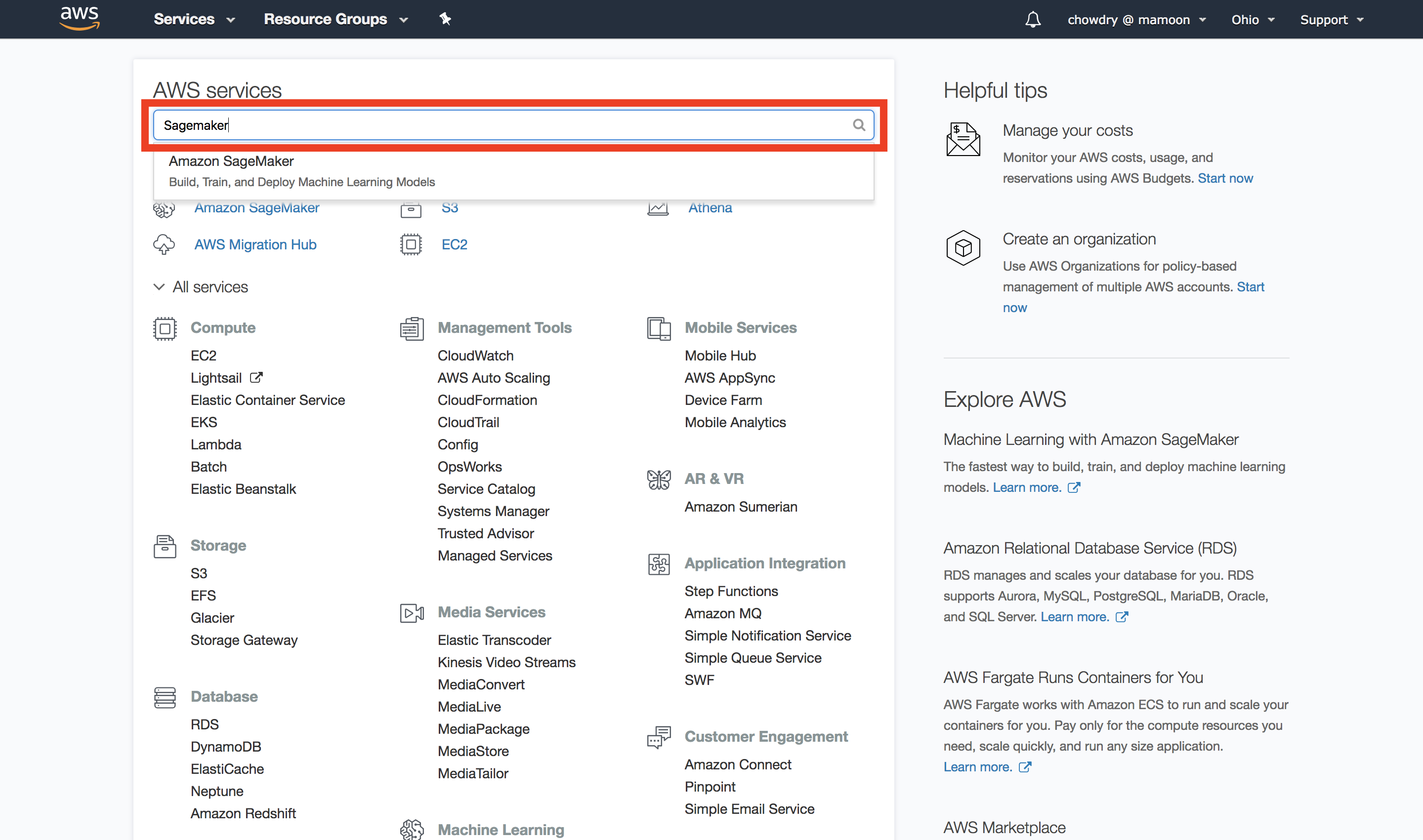
Open the AWS Management Console, so you can keep this step-by-step guide open. When the screen loads, enter your user name and password to get started. Then type Sagemaker in the search bar and select Sagemaker to open the Sagemaker console.
Step 2. Set up an Amazon SageMaker notebook instance
In this step, you will set up and configure an Amazon SageMaker notebook instance. An Amazon SageMaker notebook instance is a fully managed machine learning (ML) EC2 compute instance running the Jupyter Notebook App. Amazon SageMaker manages creating the instance and related resources. On this instance, you can create one or more Jupyter notebooks. Jupyter notebooks can be used to prepare and process data, create training jobs, deploy trained models and to validate the deployed models.
a. Launch an Amazon SageMaker notebook
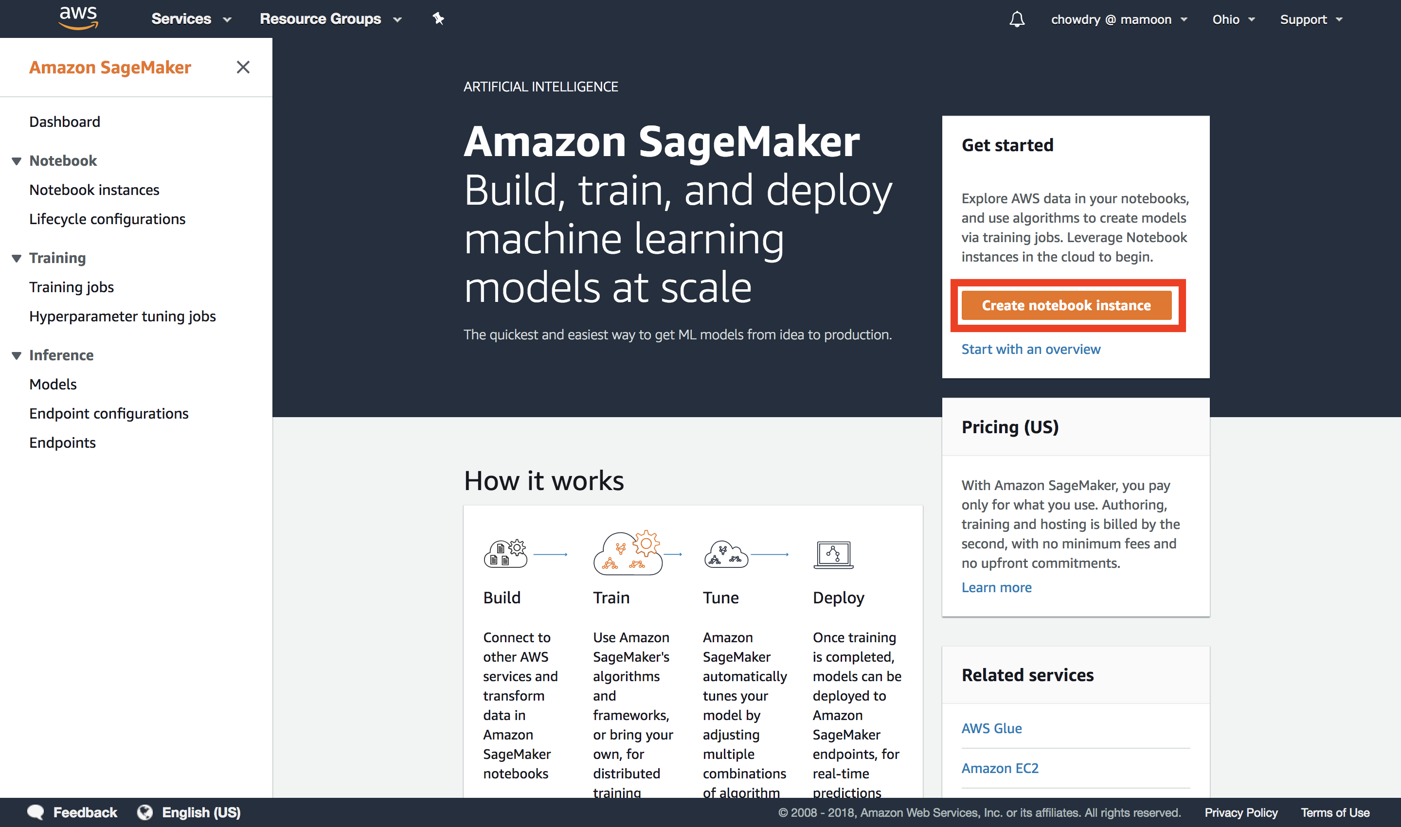
Launch an Amazon SageMaker notebook by selecting Create notebook instance in the Get started section on the right side of the screen.
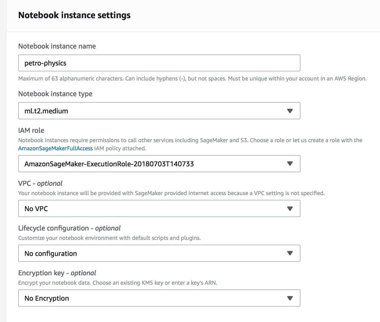
b. Complete the Notebook instance settings
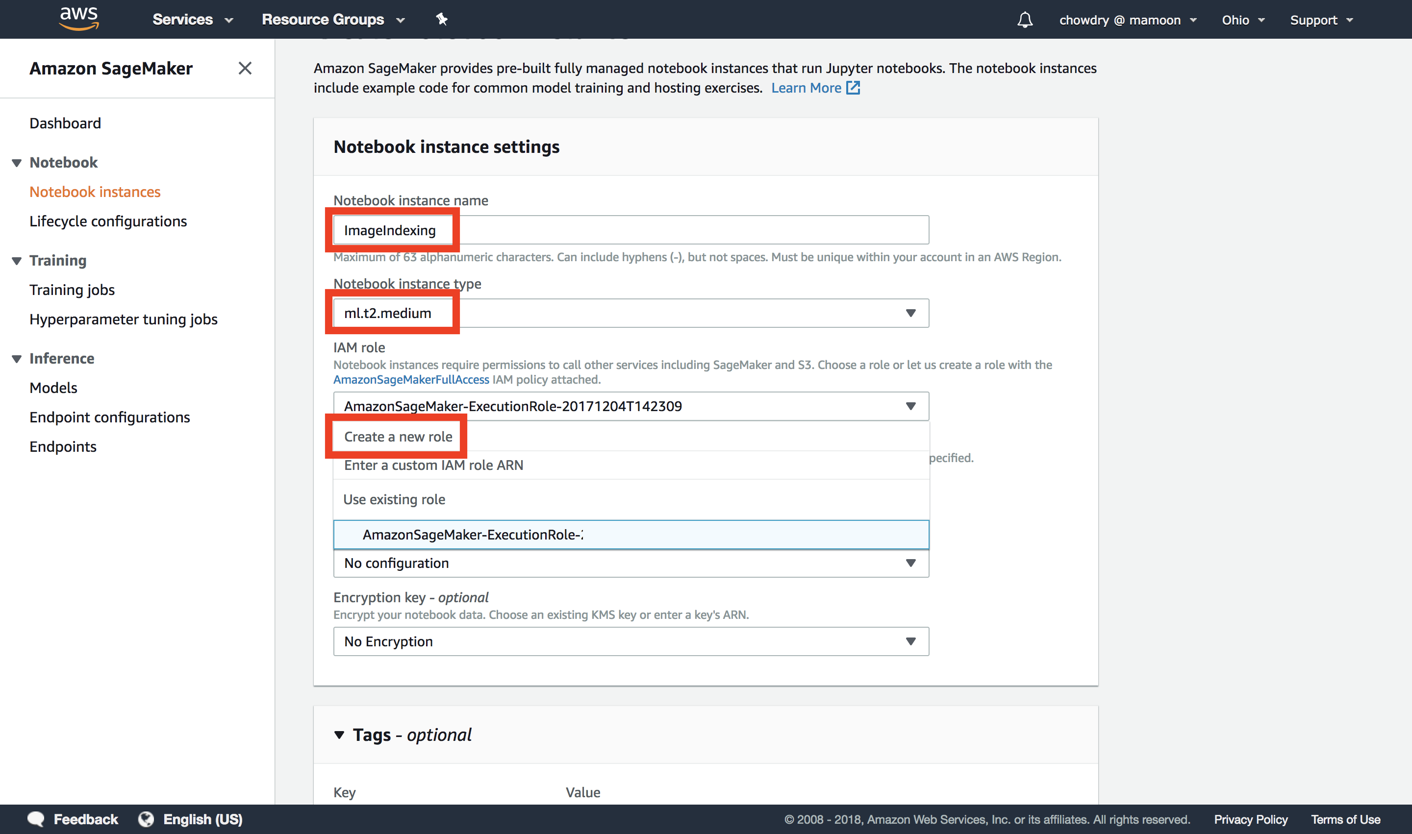
Under the Notebook instance settings section complete the following steps: 1) Give your notebook a name (for example, “ImageIndexing”), 2) Select a Notebook instance type (for example, ml.t2.medium, which is the smallest and lower cost), and 3) Select Create a new role.
c. Create a new IAM role
For IAM role, create a new role. Enter the name of the S3 bucket from Step 1 for the “Specific S3 buckets.” This IAM role allows the Amazon SageMaker Instance access to the S3 bucket containing the training data. Leave VPC, Lifecycle configuration, Encryption fields as default values. Click the “Create Notebook Instance.”
d. Wait for the notebook status to change
Wait ~2-3 minutes for the status of the notebook to change from “Pending” to “InService”
e. Open the notebook
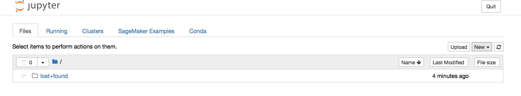
Open the notebook to see the Jupyter notebook interface.
f. Attach policies
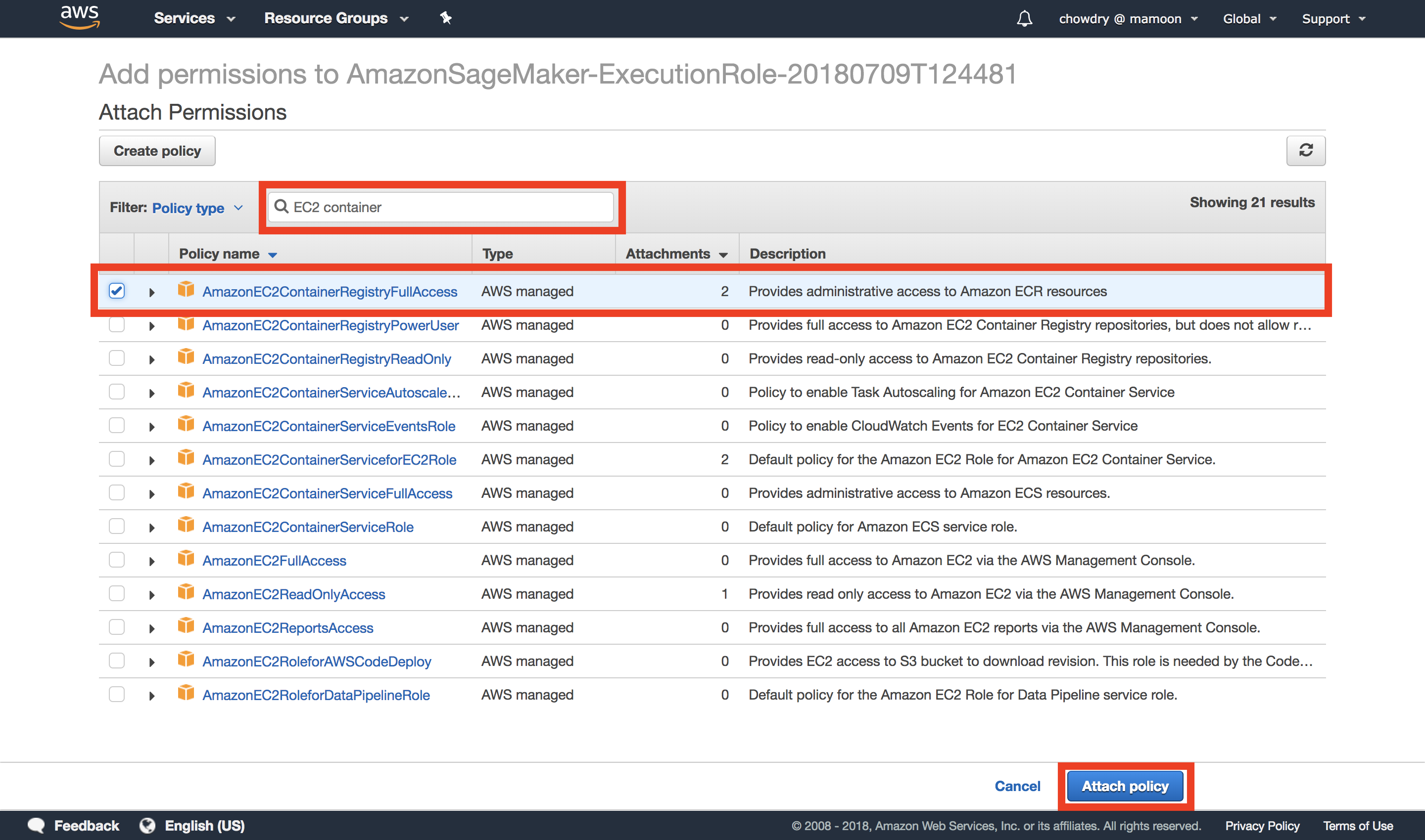
Scroll down the list of roles and select the SageMaker role that you just created. Select Attach policies.
g. Ensure the new policy has been added
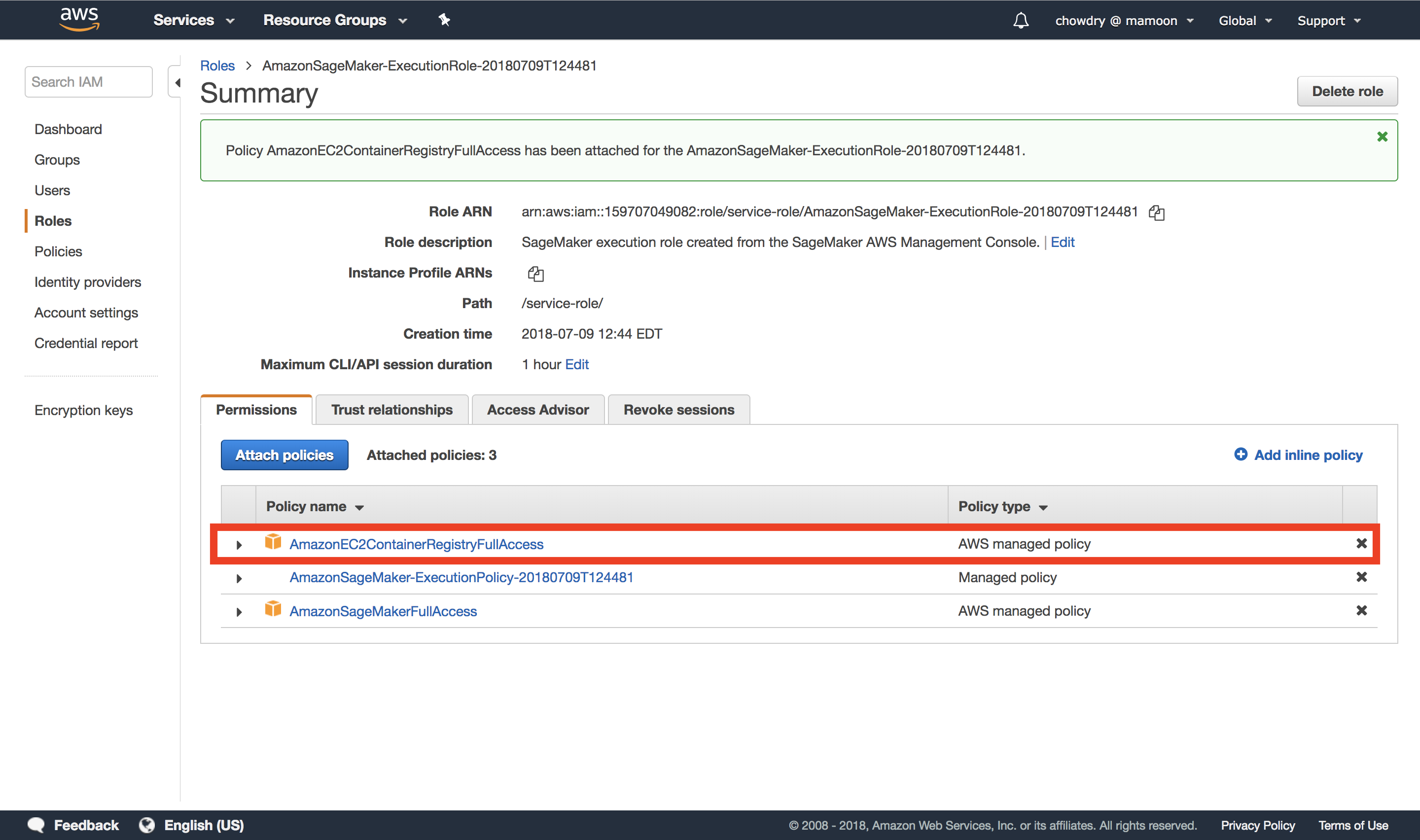
In the following summary page, ensure that the new policy has been added to the rule. Once the policy has been added, your notebook instance will have permissions to access the Amazon EC2 Container service.
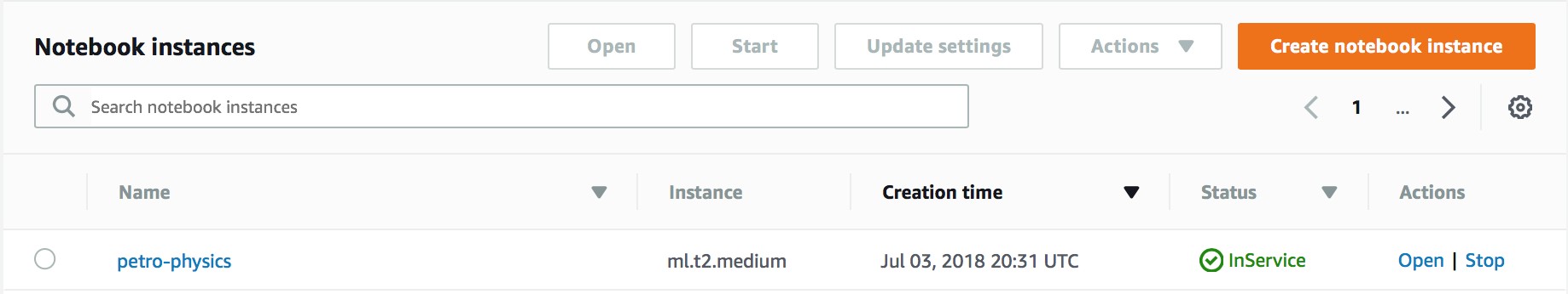
h. Return to the Amazon SageMaker Console
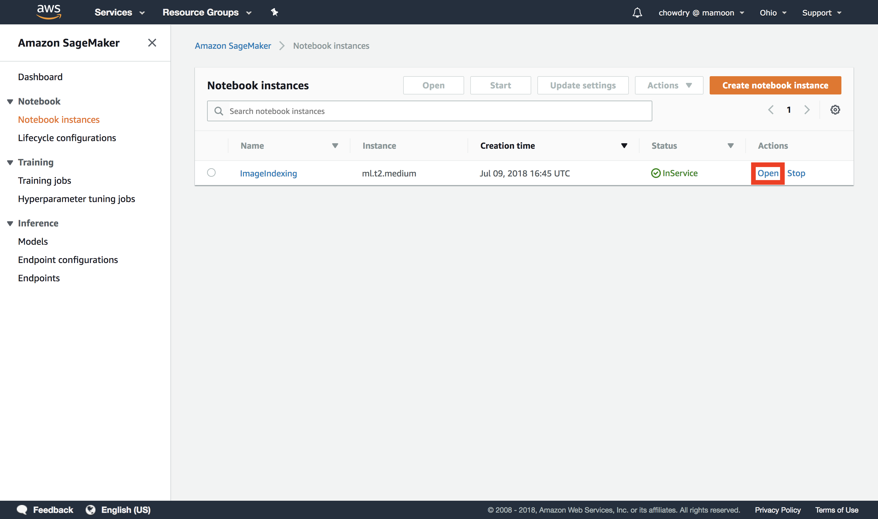
Return to the Amazon SageMaker Console and check that the notebook status is listed as InService. Once the notebook is ready, select Open. This will open the Jupyter web application on your instance.
Step 3. Configure the Jupyter Notebook
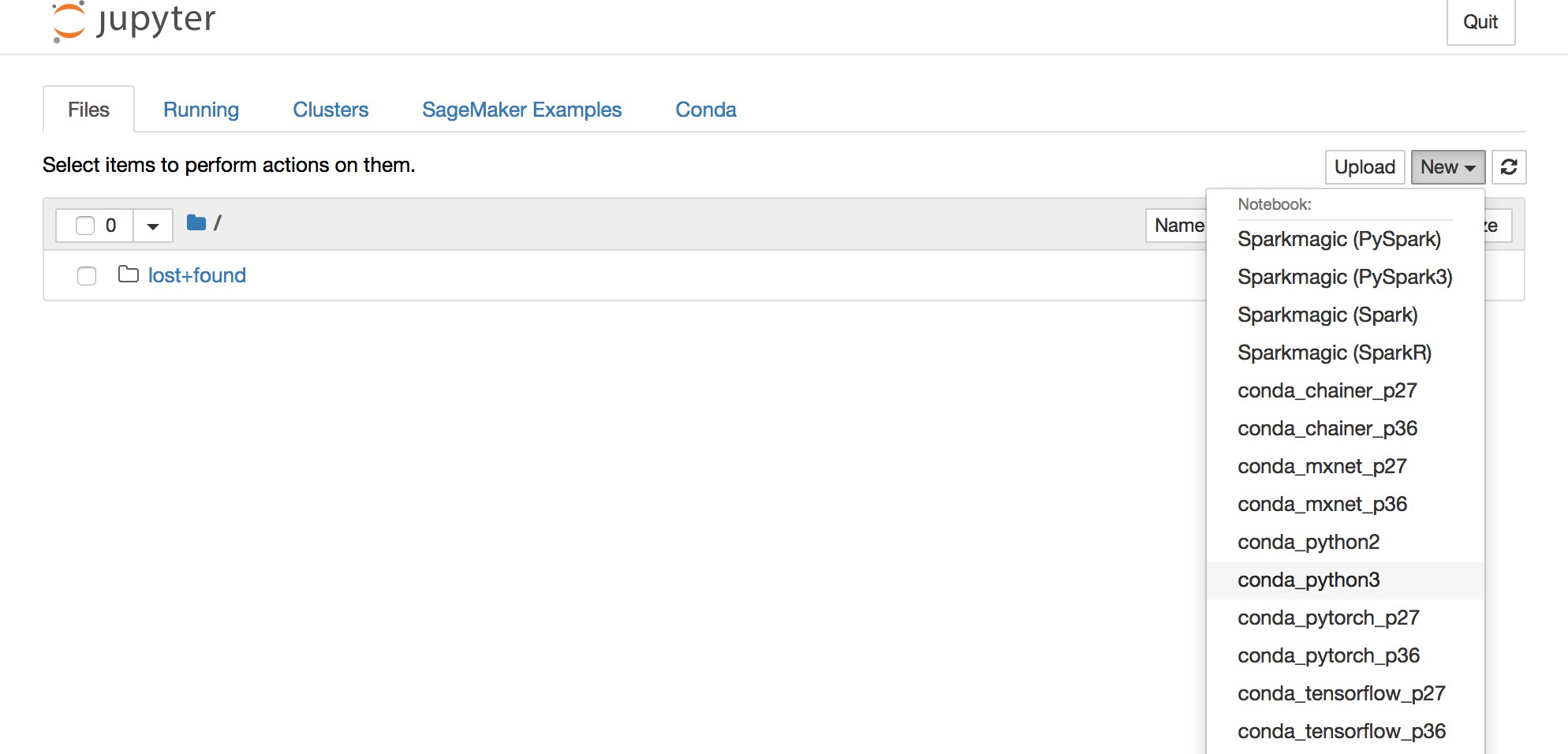
a. Set the notebook kernel
b. Rename the Untitled Jupyter notebook
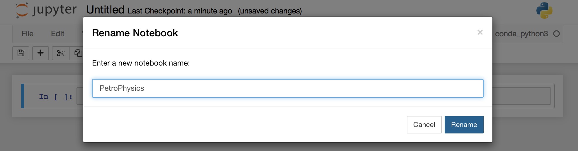
Rename the Untitled Jupyter notebook. Since multiple notebooks can be created within this instance, ensure that each notebook you created has a unique name within the instance.
c. Use Code and Markdown cells
A code cell allows you to edit and write new code, with full syntax highlighting and tab completion. When a code cell is executed, code that it contains is sent to the kernel associated with the notebook. The results that are returned from this computation are then displayed in the notebook as the cell’s output. The output is not limited to text, with many other possible forms of output are also possible, including figures and HTML tables.
You can document the computational process in a literate way, alternating descriptive text with code, using rich text. This is accomplished by marking up text with the Markdown language in the cells called Markdown cells. The Markdown language provides a simple way to perform this text markup, that is, to specify which parts of the text should be emphasized (italics), bold, form lists, etc. When a Markdown cell is executed, the Markdown code is converted into the corresponding formatted rich text. Markdown allows arbitrary HTML code for formatting.
Using the combination of code and markdown cells, you will capture the complete narrative of the use case including code and comments explaining code and results. This allows you to create and share with others, executable code and detailed documentation in a single notebook.
In the following steps, you will complete the Jupyter notebook by creating and running a combination of markdown and code cells.
Step 4A: Introduce and document the use case within Jupyter notebook
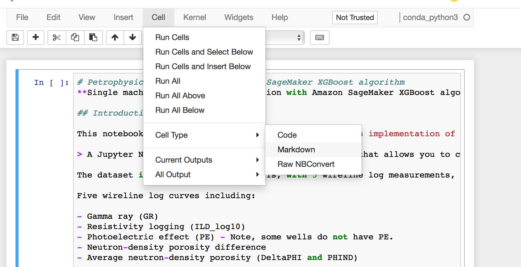
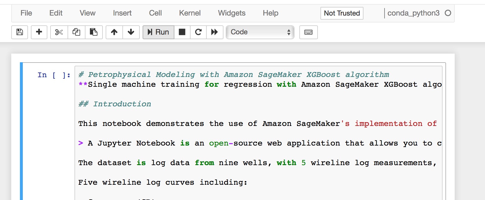
a. Enter the content below as a first cell of the notebook and change the cell type to "Markdown"
JavaScript
Single machine training for regression with Amazon SageMaker XGBoost algorithm
# Petrophysical Modeling with Amazon SageMaker XGBoost algorithm
**Single machine training for regression with Amazon SageMaker XGBoost algorithm**
## Introduction
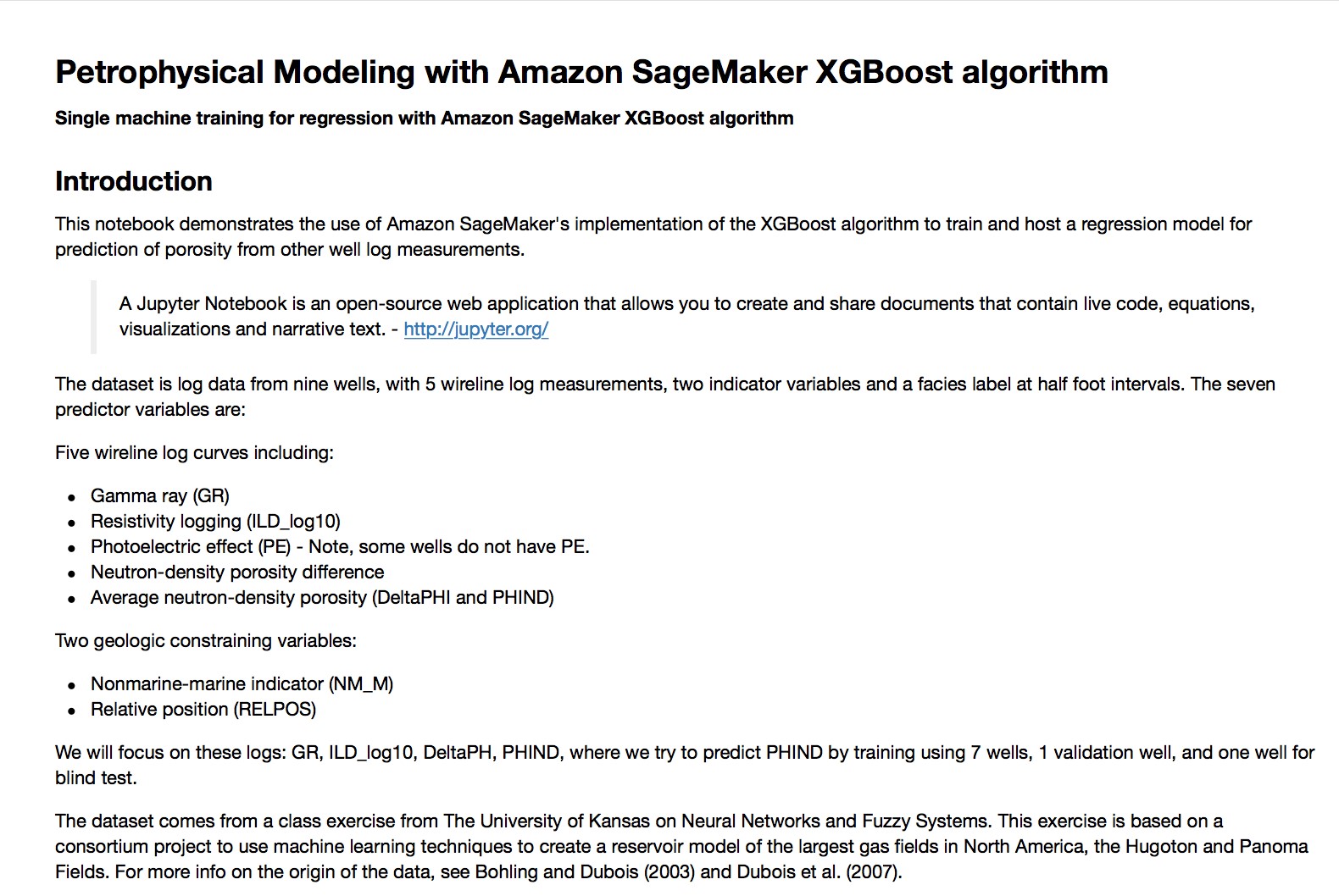
This notebook demonstrates the use of Amazon SageMaker's implementation of the XGBoost algorithm to train and host a regression model for prediction of porosity from other well log measurements.
> A Jupyter Notebook is an open-source web application that allows you to create and share documents that contain live code, equations, visualizations and narrative text. - http://jupyter.org/
The dataset is log data from nine wells, with 5 wireline log measurements, two indicator variables and a facies label at half foot intervals. The seven predictor variables are:
Five wireline log curves including:
- Gamma ray (GR)
- Resistivity logging (ILD_log10)
- Photoelectric effect (PE) - Note, some wells do not have PE.
- Neutron-density porosity difference
- Average neutron-density porosity (DeltaPHI and PHIND)
Two geologic constraining variables:
- Nonmarine-marine indicator (NM_M)
- Relative position (RELPOS)
We will focus on these logs: GR, ILD_log10, DeltaPH, PHIND, where we try to predict PHIND by training using 7 wells, 1 validation well, and one well for blind test.
The dataset comes from a class exercise from The University of Kansas on Neural Networks and Fuzzy Systems. This exercise is based on a consortium project to use machine learning techniques to create a reservoir model of the largest gas fields in North America, the Hugoton and Panoma Fields. For more info on the origin of the data, see Bohling and Dubois (2003) and Dubois et al. (2007).Step 4B: Introduce and document the use case within Jupyter notebook
a. Run the cell
Run the cell, by selecting the “Run” button from the toolbar.
b. Validate the corresponding output
Validate the corresponding output.
Step 5A. Fetch the training data and upload to S3
In the following steps, use the process explained in Step 4 to create a ‘markdown’ cell. Cells in the notebook will default to ‘Code’ cells.) a. Create and run the next cells in the notebook as a ‘markdown’
## Specify the S3 bucket to upload the training data.

Replace the ‘S3_BUCKET_NAME’ with the S3 bucket you want to use.
Step 5B. Fetch the training data and upload to S3
b. Create and run the following
%%time
import os
import boto3
import re
from sagemaker import get_execution_role

role = get_execution_role()
region = boto3.Session().region_name

bucket=’S3_BUCKET_NAME’ # NOTE : put your s3 bucket name here, and create s3 bucket
prefix = 'public-data-example/high-level’
bucket_path = 'https://s3-{}.amazonaws.com/{}'.format(region,bucket)
Step 5C. Fetch the training data and upload to S3
c. Create and run the following as ‘markdown’
### Fetching the dataset
Following methods will split the data into train/test/validation datasets and upload files to S3.
Step 5D. Fetch the training data and upload to S3
d. Create and run the next cell in the notebook with the content below:
%time

import io
import boto3
import random

# Split the data in FILE_DATA into 3 different files (FILE_TRAIN, FILE_VALIDATION, FILE_TEST)  based on well names (Valid_Well_Name and Blind_Well_Name).
def data_split(FILE_DATA, FILE_TRAIN, FILE_VALIDATION, FILE_TEST, Valid_Well_Name, Blind_Well_Name, TARGET_VAR):
    data = pd.read_csv(FILE_DATA)
    n = data.shape[0]

    # Make the first column the target feature
    cols = data.columns.tolist()
    target_pos = data.columns.get_loc(TARGET_VAR)
    cols.pop(target_pos)
    cols = [TARGET_VAR] + cols
    data = data.loc[:,cols]

    # Split data
    # Use data about the ‘Blind_Well_Name’ well as the test data.
    test_data = data[data['Well Name'] == Blind_Well_Name]
    # From the test data drop the ‘Well Name’ feature as it doesn’t add any value in the training/validation/test process.
    test_data = test_data.drop(['Well Name'], axis=1)

    # Use data about the ‘Valid_Well_Name’ well as the validation data.
    valid_data = data[data['Well Name'] == Valid_Well_Name]
	# From the valid data drop the ‘Well Name’ feature as it doesn’t add any value in the     training/validation/test process.
    valid_data = valid_data.drop(['Well Name'], axis=1)

    # Use remaining data is as the training data.
    train_data = data[data['Well Name'] != Blind_Well_Name]
    train_data = train_data[train_data['Well Name'] != Valid_Well_Name]
    # From the training data drop the ‘Well Name’ feature as it doesn’t add any value in the training/validation/test process.
    train_data = train_data.drop(['Well Name'], axis=1)

    train_data.to_csv(FILE_TRAIN, index=False, header=False)
    valid_data.to_csv(FILE_VALIDATION, index=False, header=False)
    test_data.to_csv(FILE_TEST, index=False, header=False)

def write_to_s3(fobj, bucket, key):
    return boto3.Session().resource('s3').Bucket(bucket).Object(key).upload_fileobj(fobj)

def upload_to_s3(bucket, channel, filename):
    fobj=open(filename, 'rb')
    key = prefix+'/'+channel+'/'+filename
    url = 's3://{}/{}'.format(bucket, key)
    print('Writing to {}'.format(url))
    write_to_s3(fobj, bucket, key)
    return(url)
Step 5E. Fetch the training data and upload to S3
e. Create and run the following as ‘markdown’
## Data Ingestion

Next, we read the dataset from the existing repository into memory, for preprocessing prior to training. This processing could be done in situ by Amazon Athena, Apache Spark in Amazon EMR, Amazon Redshift, etc., assuming the dataset is present in the appropriate location. Then, the next step would be to transfer the data to S3 for use in training. For small datasets, such as this one, reading into memory isn't onerous, though it would be for larger datasets.

When using the csv option, here is the critical piece of information about the data format:
For CSV training, the algorithm assumes that the target variable is in the first column and that the CSV does not have a header record. For CSV inference, the algorithm assumes that CSV input does not have the label column.
Step 5F. Fetch the training data and upload to S3
f. Upload the following training data
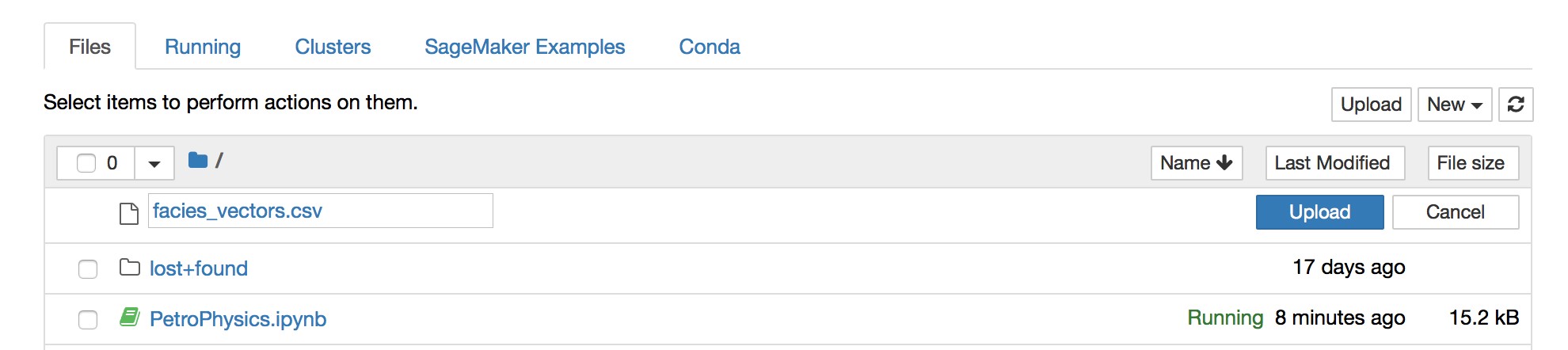
Upload the following training data from this S3 bucket: “facies_vectors.csv”
Step 5G. Fetch the training data and upload to S3
g. Run the following to remove non-numeric and empty columns and rows from training data.
# Remove non-numeric columns
import pandas as pd
data = pd.read_csv('facies_vectors.csv')
# Remove rows with missing values
data.dropna(inplace=True)

data['Well Name'].unique()
data = data.loc[:,['Well Name', 'GR', 'ILD_log10', 'DeltaPHI', 'PHIND']]

# Write file back to disk
data.to_csv('facies_num.csv', index=False)
Step 5H. Fetch the training data and upload to S3
5h. Run the following to split the dataset into training, validation and test data sets based on well names.
FILE_DATA = 'facies_num.csv'
TARGET_VAR = 'PHIND'
FILE_TRAIN = 'facies_train.csv'
FILE_VALIDATION = 'facies_validation.csv'
FILE_TEST = 'facies_test.csv'
Valid_Well_Name = 'SHRIMPLIN'
Blind_Well_Name = 'SHANKLE'

data_split(FILE_DATA, FILE_TRAIN, FILE_VALIDATION, FILE_TEST, Valid_Well_Name, Blind_Well_Name, TARGET_VAR)
Step 5I. Fetch the training data and upload to S3
i. Run the following to upload these datasets into S3.
# upload the files to the S3 bucket
s3_train_loc = upload_to_s3(bucket = bucket, channel = 'train', filename = FILE_TRAIN)
s3_valid_loc = upload_to_s3(bucket = bucket, channel = 'validation', filename = FILE_VALIDATION)
s3_test_loc = upload_to_s3(bucket = bucket, channel = 'test', filename = FILE_TEST)
Congratulations!
You have created a custom model for content-based image indexing and retrieval using Amazon SageMaker!
You can now customize this model for your own images to experiment with inferring similarity for any input image.