AWS Quantum Technologies Blog
Leveraging near-term quantum hardware for simulating high-dimensional dynamics
This post was contributed by Jiaqi Leng, Joseph Li, Xiaodi Wu
Scientists and engineers face numerous computational challenges in fields like fluid dynamics [1], modeling heat and sound propagation [2], and aircraft design [3]. Simulating partial differential equations (PDEs) in high dimensions offers a powerful approach to addressing these challenges. However, solving these high-dimensional differential equations is challenging for classical computers, as the computational complexity increases exponentially with the problem dimension. Quantum computers, capable of efficiently manipulating high-dimensional data in a non-classical way, offer potential for addressing these complex problems. Over the past decades, there has been progress in developing quantum algorithms for PDEs, including both linear and nonlinear equations [4,5,6]. However, most existing quantum algorithms rely on sophisticated input models of the problem data, such as block-encoded matrices and QRAM, which require large, fault-tolerant quantum computers and are thus unlikely to be implemented with near-term quantum hardware.
We, a group of researchers in the University of Maryland and the University of California, Berkeley, introduce a novel technique named Hamiltonian embedding [7], which aims to be a leap toward harnessing near-term quantum technology for simulating qudit Hamiltonians (e.g., high-dimensional PDEs with spatial discretization, bosonic systems, etc.) This technique allows us to map the desired simulation to a quantum evolutionary process that can be efficiently implemented with near-term quantum hardware. Upon measurement and simple post-selection, the dynamical properties of the desired high-dimensional PDE can be recovered. Notably, realizations of Hamiltonian embedding are not restricted to gate-based quantum computers.
In this post, we demonstrate the use cases of Hamiltonian embedding in both the IonQ and QuEra devices, both of which are accessible through Amazon Braket.
Hamiltonian embedding: mapping differential operators to local spin operators
To simulate differential equations on qubit-based quantum computers, it is necessary to discretize the differential equation in some way. Here, we consider the finite difference method applied to first and second order differential operators. Upon discretization, we can map the differential equation to a quantum dynamics problem via a finite-dimensional Hamiltonian called the problem Hamiltonian. For example, the evolution of a free particle is governed by the Schrödinger equation.

To discretize the (1D) Laplace operator, we can use the stencil method:

The resulting problem Hamiltonian (up to a minus sign) is a tridiagonal matrix with main diagonal elements Hj,j = -2h-2 and sub/super diagonal elements Hj,j+1=Hj+1,j=h-2. In practice, the problem Hamiltonians arising from many differential equations have the form of sparse, banded matrices (such as tridiagonal matrices) [8].
Ideally, one would like to have a quantum computer that directly simulates the time evolution of the problem Hamiltonian, without requiring any additional overhead. However, existing quantum computers are using local spin operators (i.e., Pauli matrices), and their native operators allow for only local interactions between qubits. Meanwhile, the qubit operator representation of sparse matrices often requires highly non-local interaction terms. How do we address this mismatch between the problem Hamiltonian and the device Hamiltonian?
To enable the simulation of differential equations on quantum hardware, we develop a technique known as Hamiltonian embedding. The main idea is to map the problem Hamiltonian to an embedding Hamiltonian (i.e., local spin operators) which are more easily simulated by the physical hardware. More concretely, given a target problem Hamiltonian A, we aim to design a larger operator H (called an embedding Hamiltonian) composed of local spin operators that admits a block-diagonal decomposition: H = diag(A,*), where A is embedded in the upper left corner of H. Therefore, by simulating the time evolution of H on a quantum computer —presumably easier than simulating A itself — we effectively implement the evolution of A in the upper left corner e-iHt=diag(e-iAt,*). In what follows, we present an example to illustrate the idea.
Let us consider an 8-by-8 binary-valued matrix A with all zeros except for A1,8=A8,1=1 and Aj,j+1=Aj+1,j=1 for j = 1,…,7.

This matrix is circulant and is a simple version of a Laplace operator with periodic boundary conditions. In the language of quantum computing, A corresponds to a three-qubit Hamiltonian. Although A has a simple structure, representing it as a quantum circuit (for example, using block-encoding) is challenging and may require multiple extra qubits to assist in the process [9]. If we break down A into combinations of basic Pauli strings, we end up with many component operators; some of them, like XXX, involve interactions between 3 qubits at once. This makes simulating such a seemingly simple Hamiltonian a challenge for today’s quantum computers.
Alternatively, Hamiltonian embedding allows us to represent A using only very simple quantum operations. The idea is to consider a 4-qubit Hamiltonian Sx=X1+X2+X3+X4, where each Xj is a Pauli-X operator acting on the site j. The Hilbert space of this Hamiltonian has basis. Then, we consider an 8-dimensional subspace spanned by the basis shown in Table 1 (called circulant unary code, see Sec. B.2.1 in [7]):
| Circulant unary code (N = 8) | |||
|---|---|---|---|
| Basis Index | Codeword | Basis Index | Codeword |
| 1 | 0000 | 5 | 1111 |
| 2 | 0001 | 6 | 1110 |
| 3 | 0011 | 7 | 1100 |
| 4 | 0111 | 8 | 1000 |
Table 1: Example of the circulant unary code for representing banded circulant matrices.
We can readily verify that projecting Sx onto this subspace yields exactly our target matrix A, as the Hamming distance between two adjacent codewords (including between 1 and 8) is always 1. By preparing an initial state within this subspace and penalizing any leakage outside of it, researchers can achieve the quantum simulation of A using a small number of elementary gates (or analog evolution time) without ancilla qubits. We post-select measurement outcomes confined to the relevant subspace, disregarding those outside of it. For this problem, alternative embedding schemes — such as those based on antiferromagnetic or one-hot codes — can achieve the same goal. For more details of the Hamiltonian embedding technique, we encourage interested readers to read the original paper [7].
Simulating 2D Schrödinger equation using QuEra
The time evolution of a quantum system in real space is described by the Schrödinger equation:

where u(t,x) is the wave function, f(x) is a potential function, and the spatial variable x is in -dimensional real space. In practice, the dimension d may be very high, corresponding to the number of electrons in quantum chemistry [10] or the dimension of complex nonlinear optimization problems [11].
In this blog, we showcase how to leverage Hamiltonian embedding to simulate the dynamics generated by a two-dimensional Schrödinger equation using real quantum computing devices. By performing spatial discretization of the system Hamiltonian
![]()
we obtain a problem Hamiltonian of the following form:
![]()
Where D is the discretized 1D Laplace operator (as discussed above), and U is a diagonal matrix corresponding to the potential field f(x,y). The size of the problem Hamiltonian is N2, where N is the discretization number per dimension.
On the QuEra device, the machine Hamiltonian is given by

Where A(t) and B(t) denote the Rabi frequency and detuning, respectively; Xj’s are the Pauli-X matrices, nj counts if the j-th qubit is in the excited state (i.e., number operator); Vij=C6/|ri – rj|6 denotes the Rydberg interaction between atoms i and j. Since the Rydberg interaction coefficient Vij must be positive, the Rydberg Hamiltonian HRyd requires a ingenious design of the embedding scheme, as the unary and one-hot embeddings cannot be straightforwardly applied. In order to match the device Hamiltonian, we devise an embedding scheme which we call the antiferromagnetic embedding. Intuitively, this encoding allows us to label the states using domain walls in an antiferromagnet (i.e., two neighboring qubits measured in the opposite states), as given in Table 2.
| Antiferromagnetic code (N = 7) | |||
|---|---|---|---|
| Basis Index | Codeword | Basis Index | Codeword |
| 1 | 010101 | 5 | 011010 |
| 2 | 010100 | 6 | 001010 |
| 3 | 010110 | 7 | 101010 |
| 4 | 010010 | ||
Table 2: Example of antiferromagnetic code for representing the real-space Schrödinger equation.
As it turns out, this embedding scheme enables us to map the problem Hamiltonian Hprob to the Rydberg Hamiltonian HRyd via a deliberate choice of the parameters A(t), B(t), and the atom locations.
In our experiment, we choose a discretization number N=7, which amounts to a total of 12 qubits, where the qubits are grouped into two chains of 6 qubits each. Each chain of qubits is used to represent a single spatial variable (x and y). With the Hamiltonian embedding, the (discretized) kinetic operator is mapped to the Pauli-X operators:

and the (discretized) potential operator is mapped to the diagonal part in the QuEra machine Hamiltonian:

Although encoding arbitrary continuous potential U requires more complex programmability than what is currently available, the native Rydberg interactions give rise to an effective potential field with checkerboard-like pattern. In Figure 1, we demonstrate the quantum simulation results on QuEra at various times. The 3D bar plot shows the quantum wave packets at T = 0.5, 1, 1.5, where the QuEra results are obtained by performing computational basis measurement. Despite some hardware-induced noise, our experimental results show a qualitative match between the QuEra device and the numerical simulation.
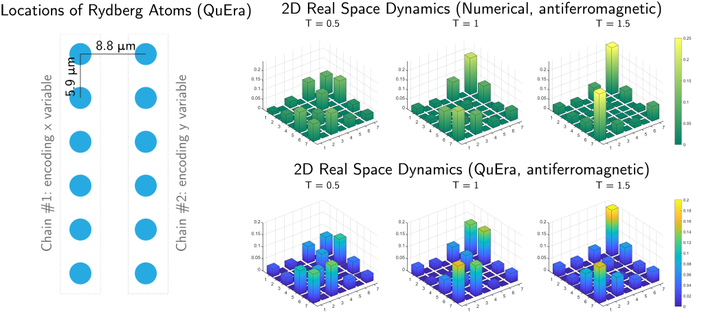
Figure 1 – Setup and results for simulating 2D Schrödinger equation using QuEra. Rydberg atom positions in the experiment¬ (left), measurement resu¬lts from numerical simulation (top right) and experiment results obtained from QuEra Aquila (bottom right). Taken from [7].
Simulating 1D Schrödinger equation using IonQ
In the previous experiment, the engineering of the potential field U is heavily restricted by the neutral atom configuration. We now demonstrate the simulation of Schrödinger equations with more structured potentials. For demonstration purposes, we illustrate how to simulate a one-dimensional Schrödinger equation on IonQ’s 25-qubit trapped ion quantum computer. It is worth noting that our method can be readily generalized to arbitrary spatial dimensions with only polynomial overheads in the dimension of the Schrödinger equations.
We consider a quantum Hamiltonian for a single bosonic mode:
![]()
The corresponding Schrödinger equation is defined over the real line. Due to the unbounded physical space, we map the physical Hamiltonian Hbs to a finite-dimensional tridiagonal matrix using a method known as Fock space truncation (a different method than the previously used spatial discretization). To map this matrix (i.e., the problem Hamiltonian) to one that is more easily implemented on IonQ, we use the one-hot embedding. Intuitively, the one-hot embedding makes use of the location of a single excitation to determine which state the system is in. Importantly, the use of Hamiltonian embedding gives us an embedding Hamiltonian which involves at most two-qubit operators (such as XX interactions). While one-hot embedding is known to be less compact and does not lead to speedups in one spatial dimension, our Hamiltonian embedding framework allows us to leverage the natural tensor structure in the Schrödinger equation. As a result, to simulate a Schrödinger equation in d dimensions, we only require O(d) qubits and polynomial-in-d interactions terms, yielding an exponential quantum advantage over naïve mesh-based approaches to PDE simulation.
The resulting embedding Hamiltonian contains up to 2-body interaction terms, which is suitable for near-term devices. More importantly, the embedding Hamiltonian can be split into a sum of an ‘’off-diagonal’’ part and a ‘’diagonal’’ part: the ‘’off-diagonal’’ part can be directly implemented using the Mølmer–Sørensen gate (native to IonQ), and the ‘’diagonal part” can be realized by parameterized single-qubit Z rotations. Since both Hamiltonian components preserve the number of excitations, by Trotterizing the dynamics, we effectively implement flip-flop dynamics that approximately simulate the 1D bosonic Hamiltonian Hbs. For details, we refer the readers to Sec. 3.4 in [7].
In our experiment, we truncate the Fock space to 5 levels and simulate a one-dimensional example. The initial state is a Gaussian distribution centered at 0 and the potential field is a quadratic function centered at 0.25. The wave function oscillates left and right over time, and we can simulate the dynamics for various time points to observe its behavior. The position and momentum operators are embedded using both XX and Z operators, so we perform observable measurements in both bases to compute their expectation values (Figure 2). Although there is substantial error due to noisy gates, we still observe the same oscillating behavior in our experiments as predicted by analytical closed-form solutions.
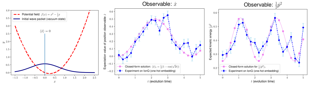
Figure 2 – Problem setup and results for real-space quantum simulation on IonQ Aria-1. As shown in the leftmost figure, the initial state is a Gaussian distribution centered at 0, and the potential field is a parabola centered at 0.25. Experiment results for the expected position (middle) and kinetic energy (right) are shown in blue, with the closed form solutions shown in pink. Taken from [4].
Discussion and outlook
We have shown how our Hamiltonian embedding technique expands the realm of quantum applications on near-term hardware. Our experiments demonstrate the first steps towards simulating high-dimensional differential equations, one of the most anticipated practical applications of quantum computers. Since the technique is broadly applicable to both analog and digital quantum computers, we expect that Hamiltonian embedding can enable quantum applications both on near-term devices and in the future with the rapid advancement of quantum technologies. Beyond quantum dynamics problems, we are excited to see how Hamiltonian embedding can accelerate practical implementations of quantum computing applications in other domains.
References
[1] Kundu P. K., Cohen I.M., Dowling D.R., & Capecelatro J. (2024). Fluid mechanics. Elsevier.
[2] Evans, L. C. (2022). Partial differential equations. American Mathematical Society.
[3] Anderson, J. (2011). Fundamentals of Aerodynamics (SI units). McGraw hill.
[4] Childs, A. M., Liu, J. P., & Ostrander, A. (2021). High-precision quantum algorithms for partial differential equations. Quantum, 5, 574.
[5] Liu, J. P., Kolden, H. Ø., Krovi, H. K., Loureiro, N. F., Trivisa, K., & Childs, A. M. (2021). Efficient quantum algorithm for dissipative nonlinear differential equations. Proceedings of the National Academy of Sciences, 118(35).
[6] Jin, S., & Liu, N. (2022). Quantum algorithms for computing observables of nonlinear partial differential equations. arXiv preprint arXiv:2202.07834.
[7] Leng, J., Li, J., Peng, Y., & Wu, X. (2024). Expanding Hardware-Efficiently Manipulable Hilbert Space via Hamiltonian Embedding. Quantum, 9, 1857.
[8] Morton, K. W., & Mayers, D. F. (2005). Numerical solution of partial differential equations: an introduction. Cambridge university press.
[9] Camps, D., Lin, L., Van Beeumen, R., & Yang, C. (2024). Explicit quantum circuits for block encodings of certain sparse matrices. SIAM Journal on Matrix Analysis and Applications, 45(1), 801-827.
[10] Babbush, R., Berry, D. W., McClean, J. R., & Neven, H. (2019). Quantum simulation of chemistry with sublinear scaling in basis size. npj Quantum Information, 5(1), 92.
[11] Leng, J., Hickman, E., Li, J., & Wu, X. (2023). Quantum Hamiltonian Descent. arXiv preprint arXiv:2303.01471.