Get started with Amazon SageMaker geospatial capabilities
Introduction
Implementation
Set up your Amazon SageMaker Studio domain
In this tutorial, you will use Amazon SageMaker Studio to access Amazon SageMaker geospatial capabilities.
Amazon SageMaker Studio is an integrated development environment (IDE) that provides a single web-based visual interface where you can access purpose-built tools to perform all machine learning (ML) development steps, from preparing data to building, training, and deploying your ML models.
If you already have a SageMaker Studio domain in the US West (Oregon) Region, follow the SageMaker Studio setup guide to attach the required AWS IAM policies to your SageMaker Studio account, then skip Step 1, and proceed directly to Step 2.
If you don't have an existing SageMaker Studio domain, continue with Step 1 to run an AWS CloudFormation template that creates a SageMaker Studio domain and adds the permissions required for the rest of this tutorial.
1. Launch the stack
Choose the AWS CloudFormation stack link.
This link opens the AWS CloudFormation console and creates your SageMaker Studio domain and a user named studio-user. It also adds the required permissions to your SageMaker Studio account.
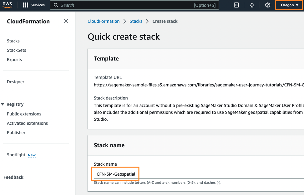
In the CloudFormation console, confirm that US West (Oregon) is the Region displayed in the upper right corner.
Stack name should be CFN-SM-Geospatial, and should not be changed. This stack takes about 10 minutes to create all the resources.
This stack assumes that you already have a public VPC set up in your account. If you do not have a public VPC, see VPC with a single public subnet to learn how to create a public VPC.
2. Confirm creation
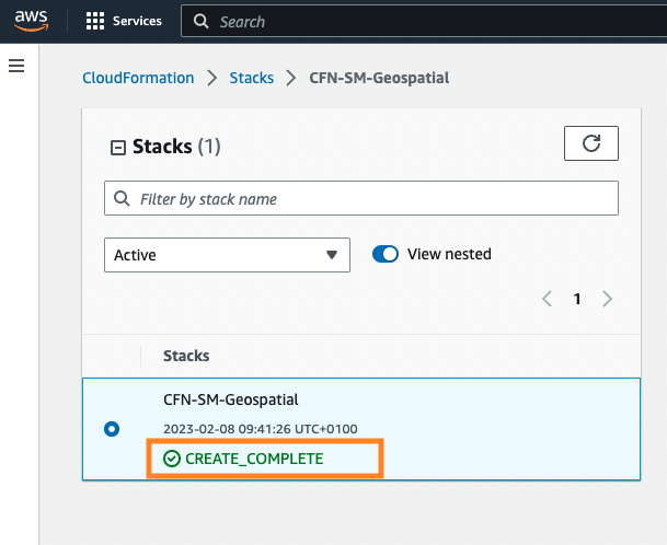
When the stack creation has been completed, you can proceed to the next section to set up a SageMaker Studio notebook.
Set up a SageMaker Studio notebook
In this step, you'll launch a new SageMaker Studio notebook with a SageMaker geospatial image, which is a Python image consisting of commonly used geospatial libraries such as GDAL, Fiona, GeoPandas, Shapely, and Rasterio, and allows you to visualize geospatial data within SageMaker.
1. Open SageMaker Studio
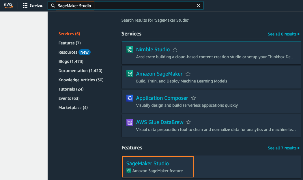
Enter SageMaker Studio into the console search bar, and then choose SageMaker Studio.
2. Choose a region
Choose US West (Oregon) from the Region dropdown list on the upper right corner of the SageMaker console.

3. Choose Open Studio
To launch the app, select Studio from the left console and select Open Studio using the studio-user profile.

4. Wait for application to launch
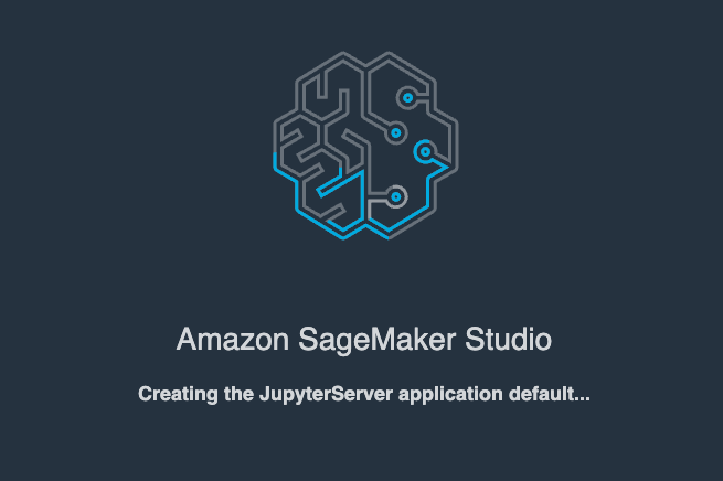
The SageMaker Studio Creating application screen will be displayed.
The application will take a few minutes to load.
5. Create a notebook
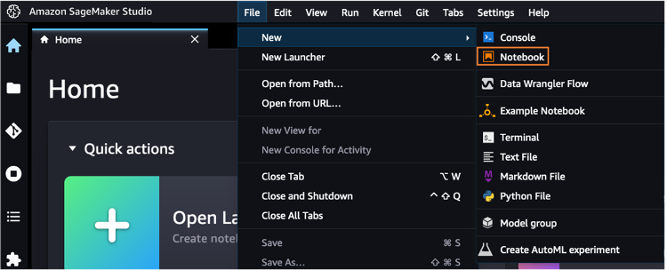
Open the SageMaker Studio interface. On the navigation bar, choose File > New > Notebook.
6. Set up environment
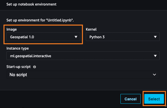
In the Set up notebook environment dialog box, under Image, select Geospatial 1.0.
The Python 3 kernel is selected automatically. Under Instance type, choose ml.geospatial.interactive.
Then, choose Select.
7. Verify kernel started
Wait until the notebook kernel has been started.

8. Verify Geospatial 1.0 shows
The kernel on the top right corner of the notebook should now display Geospatial 1.0.

Create an Earth Observation Job
In this step, you'll use Amazon SageMaker Studio geospatial notebook to create an Earth Observation job (EOJ) which allows you to acquire, transform, and visualize geospatial data.
In this example, you'll be using a pre-trained machine learning model for land cover segmentation. Depending on your use case, you can choose from a variety of operations and models when running an EOJ.
1. Initialize the geospatial client
In the Jupyter notebook, in a new code cell, copy and paste the following code and select Run.
This will initialize the geospatial client and import libraries for geospatial processing.
As the geospatial notebook image comes with these libraries already pre-installed and configured, there is no need to install them first.

Initialization code
Add this code to your notebook
import boto3
import sagemaker
import sagemaker_geospatial_map

import time
import datetime
import os
from glob import glob
import rasterio
from rasterio.plot import show
import matplotlib.colors
import matplotlib.patches as mpatches
import matplotlib.pyplot as plt
import numpy as np
import tifffile

sagemaker_session = sagemaker.Session()
export_bucket = sagemaker_session.default_bucket() # Alternatively you can use your custom bucket here.

session = boto3.Session()
execution_role = sagemaker.get_execution_role()
geospatial_client = session.client(service_name="sagemaker-geospatial")
2. Start a new Earth Oberservation Job
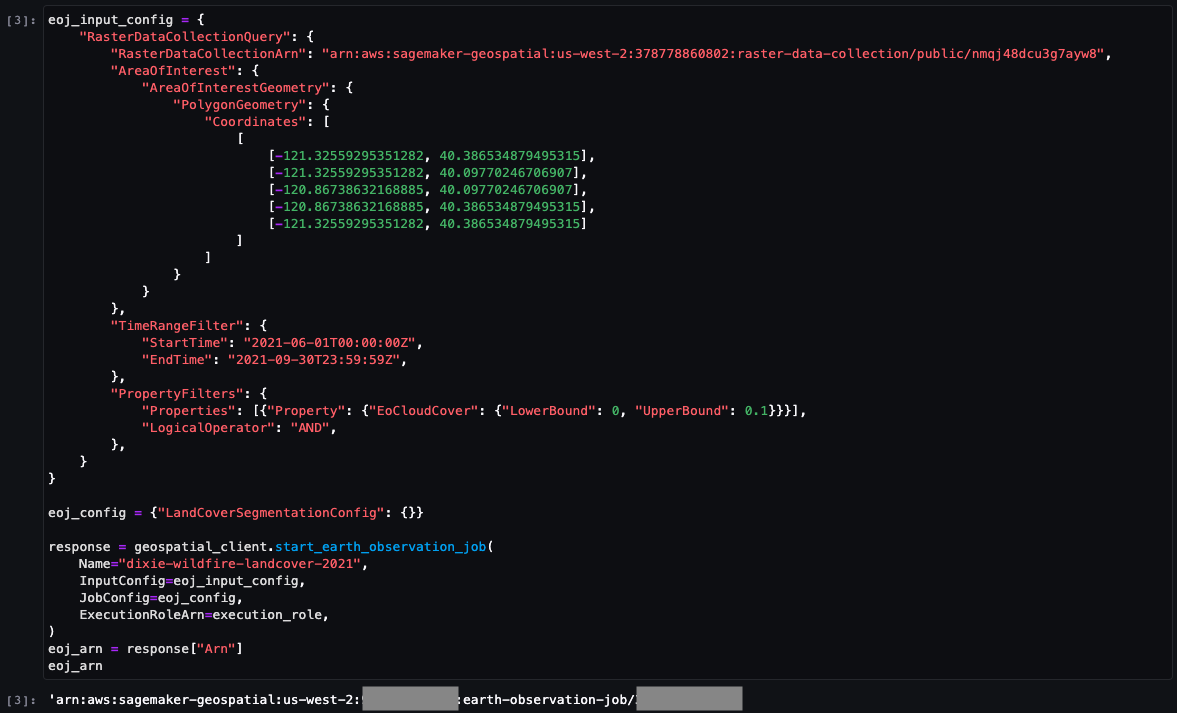
Next you will define and start a new Earth Observation Job (EOJ).
In the EOJ configuration, you can define an area of interest (AOI), a time range and cloud-cover-percentage-based filters. Also, you can choose a data provider.
In the provided configuration, the area of interest is an area in California which was affected by the Dixie wildfire. The underlying data is from the Sentinel-2 mission.
Copy and paste the following code into a new code cell. Then, select Run.
When the job is created, it can be referenced with a dedicated ARN.
EOJ code
Add this code to your notebook
eoj_input_config = {
    "RasterDataCollectionQuery": {
        "RasterDataCollectionArn": "arn:aws:sagemaker-geospatial:us-west-2:378778860802:raster-data-collection/public/nmqj48dcu3g7ayw8",
        "AreaOfInterest": {
            "AreaOfInterestGeometry": {
                "PolygonGeometry": {
                    "Coordinates": [
                        [
                            [-121.32559295351282, 40.386534879495315],
                            [-121.32559295351282, 40.09770246706907],
                            [-120.86738632168885, 40.09770246706907],
                            [-120.86738632168885, 40.386534879495315],
                            [-121.32559295351282, 40.386534879495315]
                        ]
                    ]
                }
            }
        },
        "TimeRangeFilter": {
            "StartTime": "2021-06-01T00:00:00Z",
            "EndTime": "2021-09-30T23:59:59Z",
        },
        "PropertyFilters": {
            "Properties": [{"Property": {"EoCloudCover": {"LowerBound": 0, "UpperBound": 0.1}}}],
            "LogicalOperator": "AND",
        },
    }
}

eoj_config = {"LandCoverSegmentationConfig": {}}

response = geospatial_client.start_earth_observation_job(
    Name="dixie-wildfire-landcover-2021",
    InputConfig=eoj_input_config,
    JobConfig=eoj_config,
    ExecutionRoleArn=execution_role,
)
eoj_arn = response["Arn"]
eoj_arn
3. Explore the raster data
While the job is running, you can explore the raster data which is used as input for the EOJ.
Use the geospatial SDK to retrieve image URLs in a cloud optimized GeoTIFF (COG) format.
Copy and paste the following code into a new code cell. Then, select Run.

Image retrieval code
Add this code to explore the raster data
search_params = eoj_input_config.copy()
search_params["Arn"] = "arn:aws:sagemaker-geospatial:us-west-2:378778860802:raster-data-collection/public/nmqj48dcu3g7ayw8"
search_params["RasterDataCollectionQuery"].pop("RasterDataCollectionArn", None)
search_params["RasterDataCollectionQuery"]["BandFilter"] = ["visual"]

cog_urls = []
search_result = geospatial_client.search_raster_data_collection(**search_params)
for item in search_result["Items"]:
    asset_url = item["Assets"]["visual"]["Href"]
    cog_urls.append(asset_url)

cog_urls
4. Visualize input data
Next, you will use the COG URLs to visualize the input data for the area of interest.
This provides you with a visual comparison of the area before and after the wildfire.
Copy and paste the following code into a new code cell. Then, select Run.
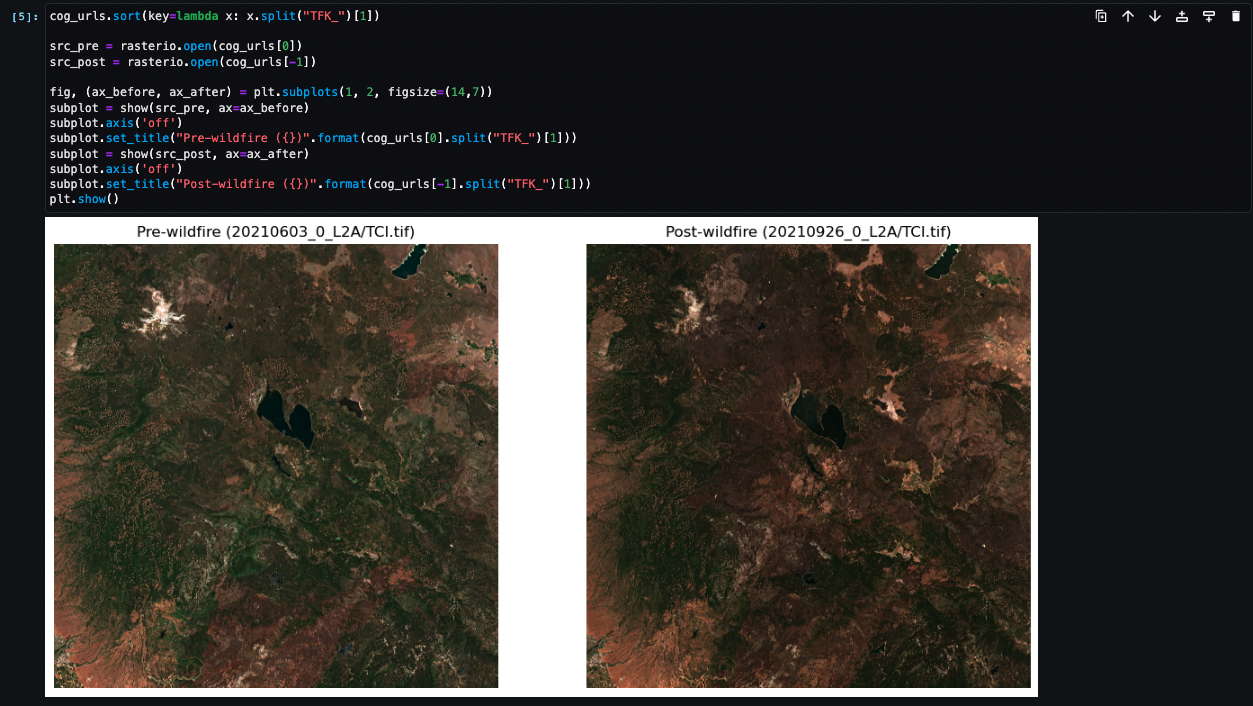
Data visualization code
Add this code to your notebook
cog_urls.sort(key=lambda x: x.split("TFK_")[1])

src_pre = rasterio.open(cog_urls[0])
src_post = rasterio.open(cog_urls[-1])

fig, (ax_before, ax_after) = plt.subplots(1, 2, figsize=(14,7))
subplot = show(src_pre, ax=ax_before)
subplot.axis('off')
subplot.set_title("Pre-wildfire ({})".format(cog_urls[0].split("TFK_")[1]))
subplot = show(src_post, ax=ax_after)
subplot.axis('off')
subplot.set_title("Post-wildfire ({})".format(cog_urls[-1].split("TFK_")[1]))
plt.show()
5. Output job status
Before you can proceed with further steps, the EOJ needs to complete.
Copy and paste the following code into a new code cell. Then, select Run.
This code will continuously output the current status of the job and execute until the EOJ is complete.
Wait until the displayed status has changed to COMPLETED. This might take up to 20-25 minutes.

Code to output job status
Add this code to your notebook
# check status of created Earth Observation Job and wait until it is completed
eoj_completed = False
while not eoj_completed:
    response = geospatial_client.get_earth_observation_job(Arn=eoj_arn)
    print("Earth Observation Job status: {} (Last update: {})".format(response['Status'], datetime.datetime.now()), end='\r')
    eoj_completed = True if response['Status'] == 'COMPLETED' else False
    if not eoj_completed:
        time.sleep(30)
Visualize the Earth Observation Job
In this step, you'll use visualization functionalities provided by Amazon SageMaker geospatial capabilities to visualize the input and outputs of your Earth Observation Job.
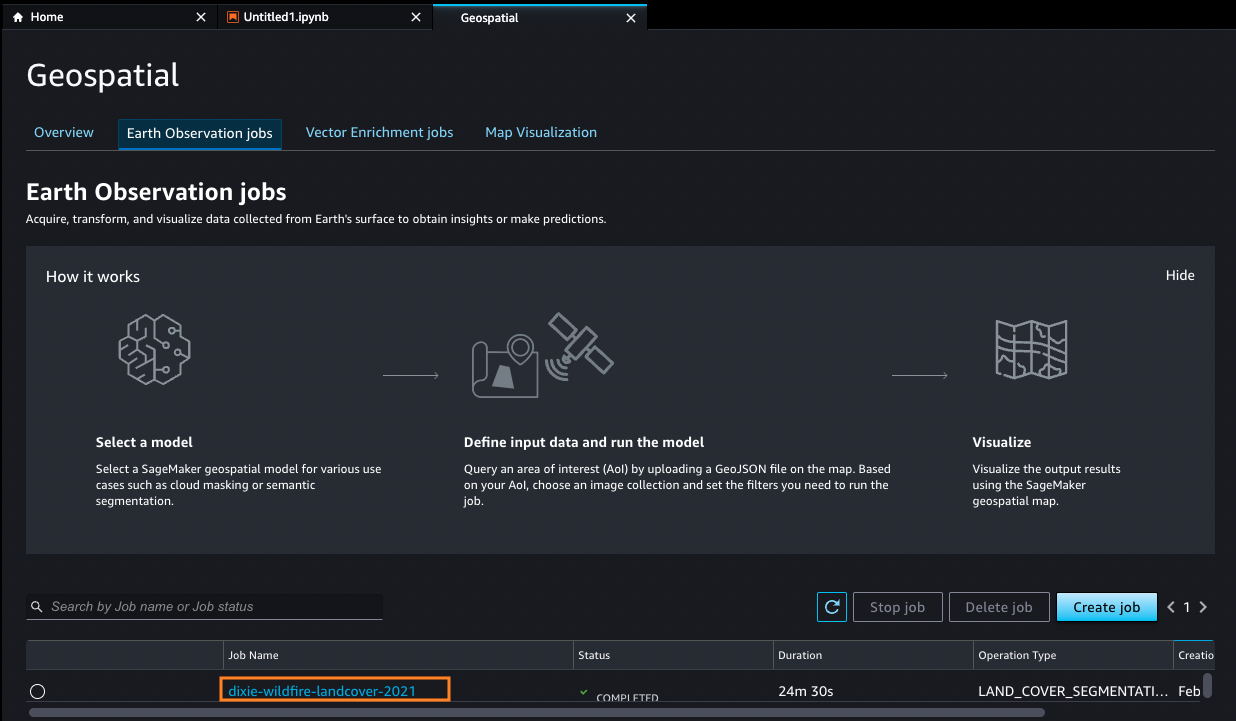
2. Select the applicable EOJ
In the new Geospatial tab, you will find an overview of all your EOJs. Select the job dixie-wildfire-landcover-2021.
3. Visualize job output
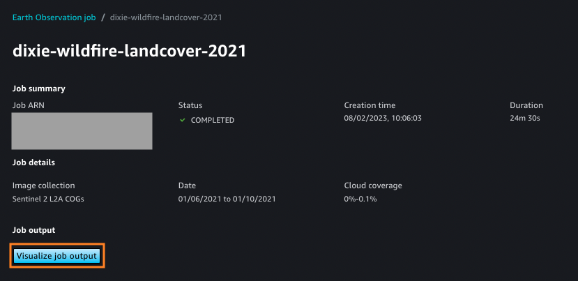
On the job detail page, choose Visualize job output.
4. View the visualization
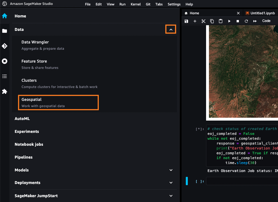
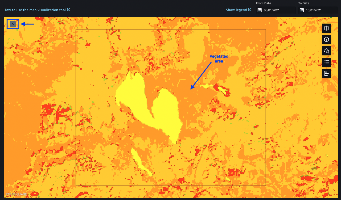
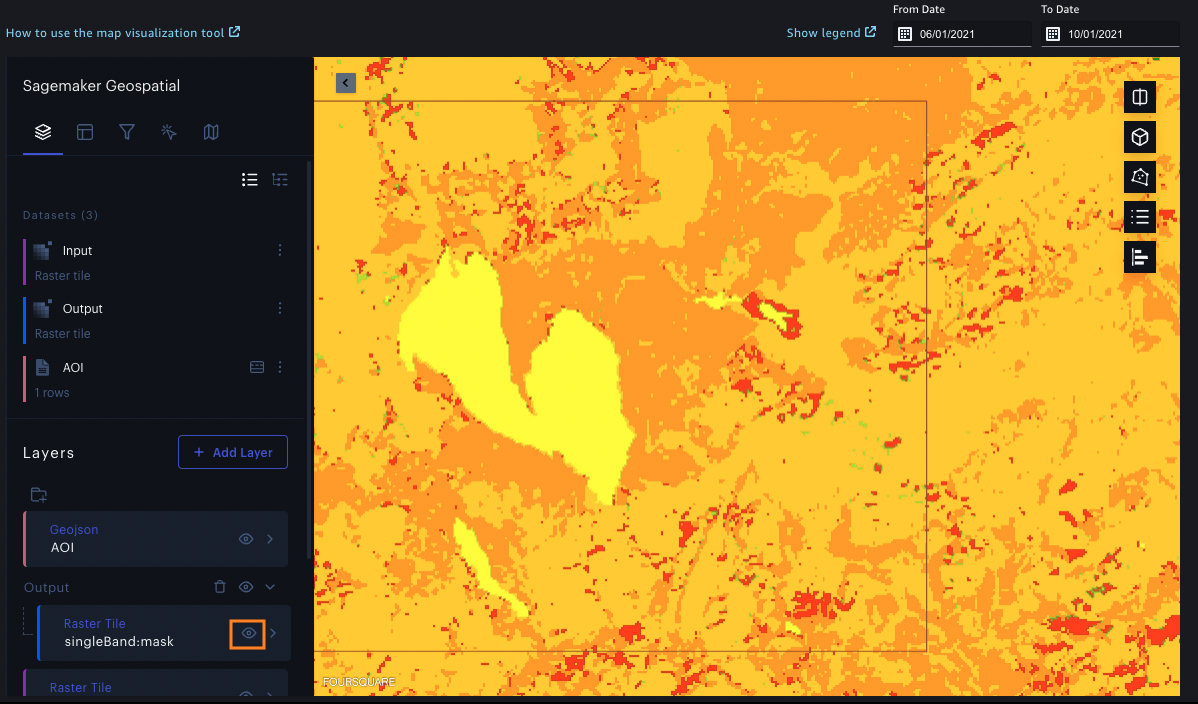
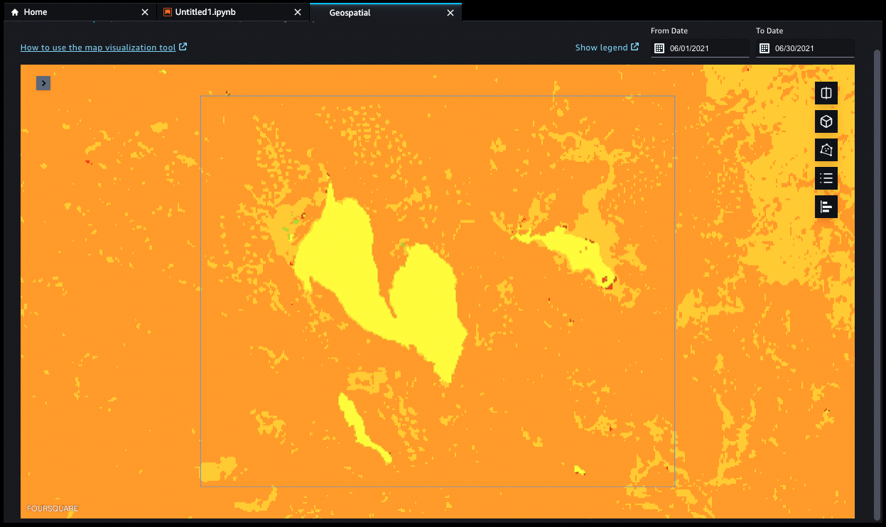
The visualization will show you the output for the landcover segmentation for the most recent date in the To Date field.
The image presented is the land cover data after the wildfire.
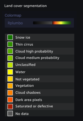
The pixels in dark orange represent vegetated areas (as described in legends for EOJ).
Select the arrow on the left side to open the visualization options.
5. Use the legend to understand the data
View the legend.
6. Configure visualization options
Within the visualization options you can select and configure all geospatial and data layers.
Select the Hide symbol for the output raster tile layer.
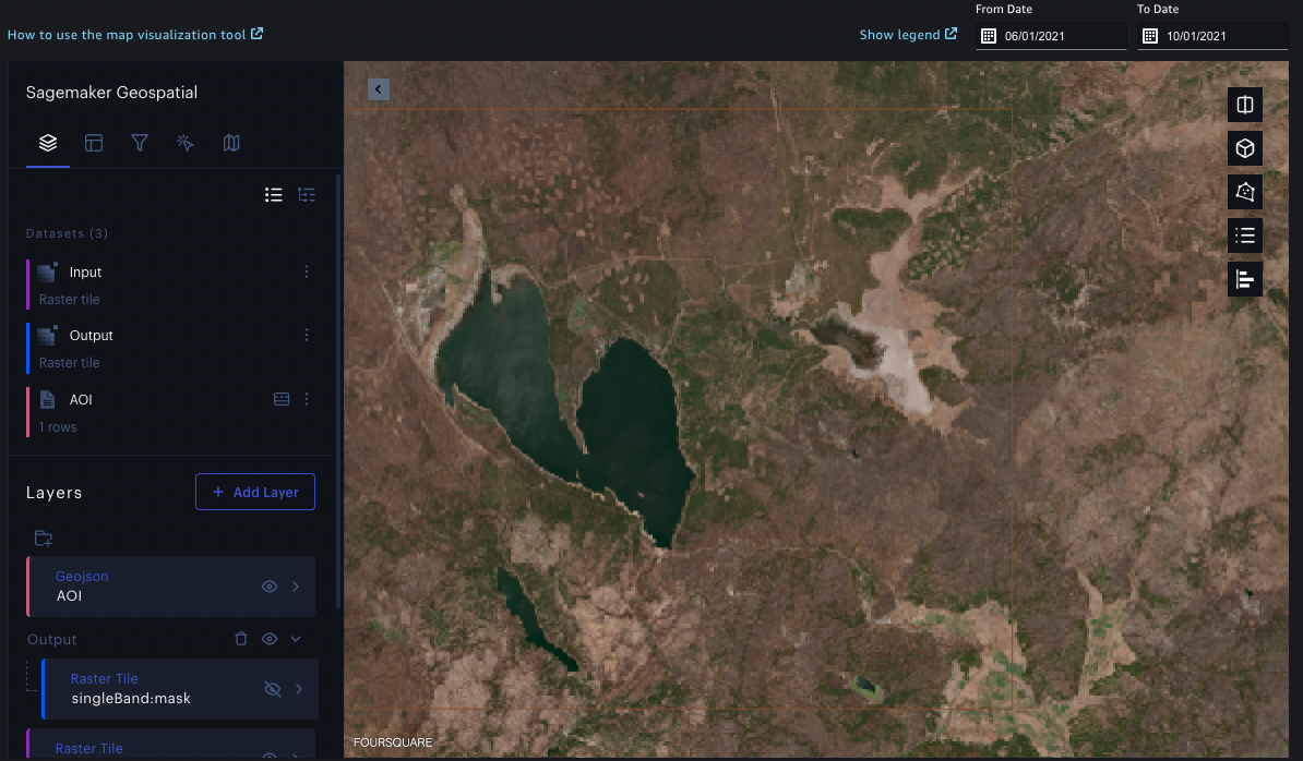
7. View the underlying input data layer
After you select the Hide symbol, you will be able to see the underlying input data layer.
8. Change the date
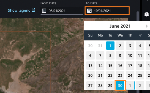
You are also able to visualize different time periods of the input and output data of your EOJ.
Select the 30th of June 2021 in the To Date field.
9. View the updated imagery
The data displayed is satellite imagery from before the 30th of June 2021.
This timeframe was before the wildfire, and the amount of vegetation (dark orange) is much higher than on the output viewed previously.
You can again select to hide the output layer to see the underlying input satellite image (as in the step before).
Export the Earth Observation Job to Amazon S3
In this step, the output data from the Earth Observation Job will be exported to an Amazon Simple Storage Service (Amazon S3) bucket and the exported segmentation masks will be downloaded for further processing.
1. Export the EOJ to S3
You will use the geospatial SDK to export the output of the Earth Observation Job to S3.
This operation takes between 1-2 minutes to complete.
Copy and paste the following code into a new code cell. Then, select Run.

Export EOJ code
Add this code to your notebook
bucket_prefix = "eoj_dixie_wildfire_landcover"
response = geospatial_client.export_earth_observation_job(
    Arn=eoj_arn,
    ExecutionRoleArn=execution_role,
    OutputConfig={
        "S3Data": {"S3Uri": f"s3://{export_bucket}/{bucket_prefix}/"}
    },
)

while not response['ExportStatus'] == 'SUCCEEDED':
    response = geospatial_client.get_earth_observation_job(Arn=eoj_arn)
    print("Export of Earth Observation Job status: {} (Last update: {})".format(response['ExportStatus'], datetime.datetime.now()), end='\r')
    if not response['ExportStatus'] == 'SUCCEEDED':
        time.sleep(30)
2. Download the mask files
Next, you will download the mask files from S3 into SageMaker Studio.
Copy and paste the following code into a new code cell. Then, select Run.

Download mask files code
Add this code to your notebook
s3_bucket = session.resource("s3").Bucket(export_bucket)

mask_dir = "./dixie-wildfire-landcover/masks"
os.makedirs(mask_dir, exist_ok=True)
for s3_object in s3_bucket.objects.filter(Prefix=bucket_prefix).all():
    path, filename = os.path.split(s3_object.key)
    if "output" in path:
        mask_local_path = mask_dir + "/" + filename
        s3_bucket.download_file(s3_object.key, mask_local_path)
        print("Downloaded mask: " + mask_local_path)

mask_files = glob(os.path.join(mask_dir, "*.tif"))
mask_files.sort(key=lambda x: x.split("TFK_")[1])
Analyze the exported segmentation masks
In this step, you'll use geospatial Python libraries included in the SageMaker geospatial image to perform further operations on the exported data.
1. Extract segmentation classes
Using the numpy and tifffile libraries, you will extract dedicated segmentation classes (vegetation and water) out of the mask data and store this data in variables for later usage.
Copy and paste the following code into a new code cell. Then, select Run.

Extract segmentation classes code
Add this code to your notebook
landcover_simple_colors = {"not vegetated": "khaki","vegetated": "olivedrab", "water": "lightsteelblue"}

def extract_masks(date_str):
    mask_file = list(filter(lambda x: date_str in x, mask_files))[0]
    mask = tifffile.imread(mask_file)
    focus_area_mask = mask[400:1100, 600:1350]

    vegetation_mask = np.isin(focus_area_mask, [4]).astype(np.uint8) # vegetation has a class index of 4
    water_mask = np.isin(focus_area_mask, [6]).astype(np.uint8) # water has a class index of 6
    water_mask[water_mask > 0] = 2
    additive_mask = np.add(vegetation_mask, water_mask).astype(np.uint8)

    return (focus_area_mask, vegetation_mask, additive_mask)

masks_20210603 = extract_masks("20210603")
masks_20210926 = extract_masks("20210926")
2. Visualize the extracted classes
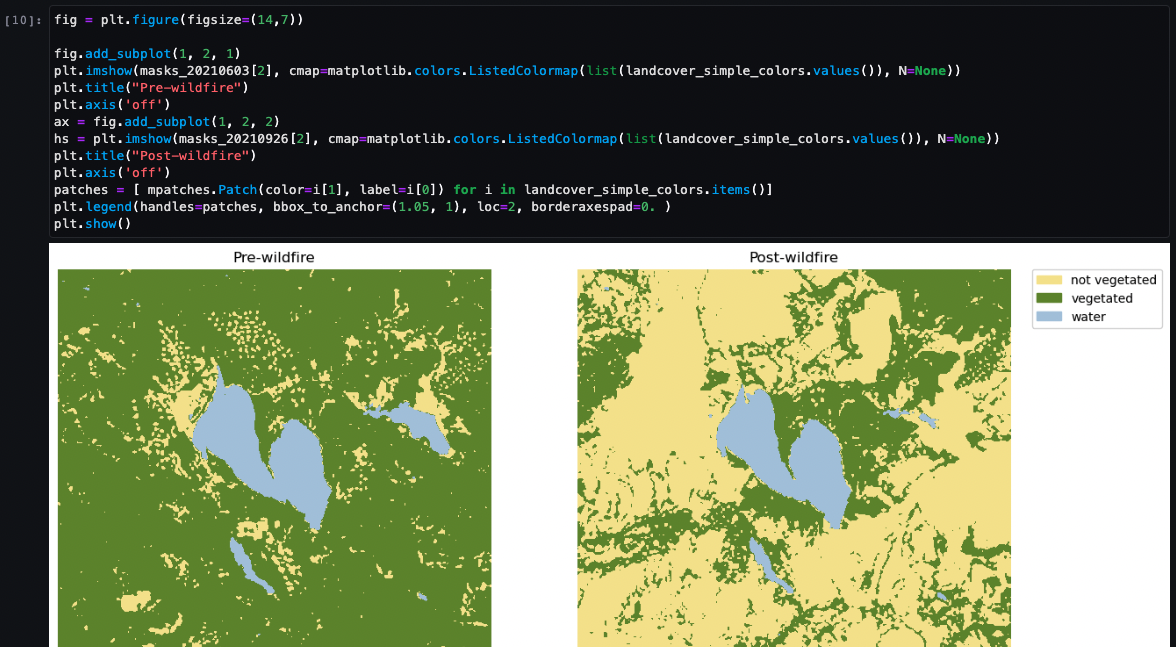
You will use now the preprocessed mask data to visualize the extracted classes.
Copy and paste the following code into a new code cell. Then, select Run.
Visualize extracted classes code
Add this code to your notebook
fig = plt.figure(figsize=(14,7))

fig.add_subplot(1, 2, 1)
plt.imshow(masks_20210603[2], cmap=matplotlib.colors.ListedColormap(list(landcover_simple_colors.values()), N=None))
plt.title("Pre-wildfire")
plt.axis('off')
ax = fig.add_subplot(1, 2, 2)
hs = plt.imshow(masks_20210926[2], cmap=matplotlib.colors.ListedColormap(list(landcover_simple_colors.values()), N=None))
plt.title("Post-wildfire")
plt.axis('off')
patches = [ mpatches.Patch(color=i[1], label=i[0]) for i in landcover_simple_colors.items()]
plt.legend(handles=patches, bbox_to_anchor=(1.05, 1), loc=2, borderaxespad=0. )
plt.show()
3. Compute and visualize the difference
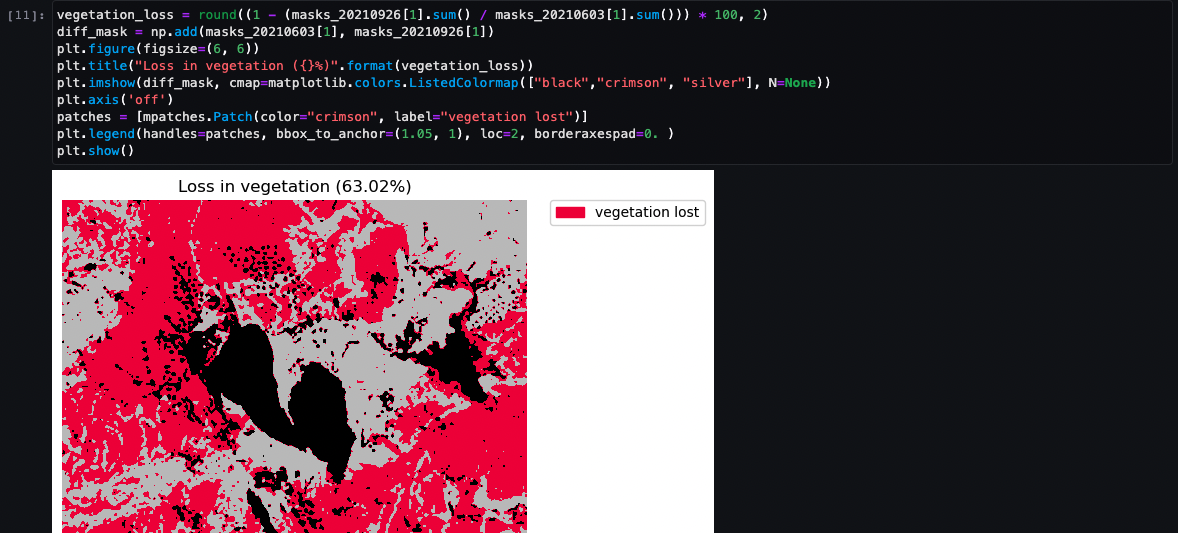
Finally, you will compute and visualize the difference between the post- and pre-wildfire mask.
This shows the impact the wildfire had on the vegetation in the observed area. More than 60% of vegetation was lost as a direct impact of the fire.
Copy and paste the following code into a new code cell. Then, select Run.
Difference computation code
Add this code to your notebook
vegetation_loss = round((1 - (masks_20210926[1].sum() / masks_20210603[1].sum())) * 100, 2)
diff_mask = np.add(masks_20210603[1], masks_20210926[1])
plt.figure(figsize=(6, 6))
plt.title("Loss in vegetation ({}%)".format(vegetation_loss))
plt.imshow(diff_mask, cmap=matplotlib.colors.ListedColormap(["black","crimson", "silver"], N=None))
plt.axis('off')
patches = [mpatches.Patch(color="crimson", label="vegetation lost")]
plt.legend(handles=patches, bbox_to_anchor=(1.05, 1), loc=2, borderaxespad=0. )
plt.show()
Clean up your AWS resources
It is a best practice to delete resources that you no longer need so that you don't incur unintended charges.
1. Delete the bucket
To delete the S3 bucket, complete the following steps:
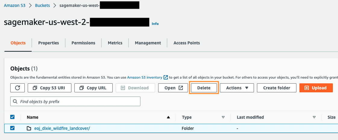
Open the Amazon S3 console. On the navigation bar, choose Buckets, sagemaker-<your-Region>-<your-account-id>, and then select the checkbox next to eoj_dixie_wildfire_landcover. Then, choose Delete.
On the Delete objects dialog box, verify that you have selected the proper object to delete and enter permanently delete into the Permanently delete objects confirmation box.
Once this is complete and the bucket is empty, you can delete the sagemaker-<your-Region>-<your-account-id> bucket by following the same steps again.
2. Choose the SageMaker Studio domain
Note: The Geospatial kernel used for running the notebook image in this tutorial will accumulate charges until you either stop the kernel or perform the following steps to delete the apps. For more information, see Shut Down Resources in the Amazon SageMaker Developer Guide.
To delete the SageMaker Studio apps, perform the following steps:
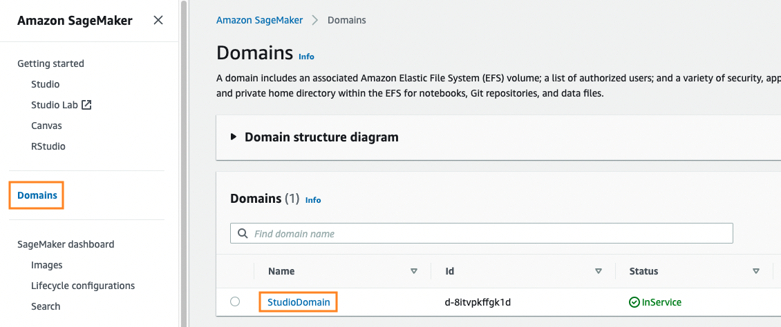
In the SageMaker console, choose Domains, and then choose StudioDomain
3. Delete the SageMaker Studio apps
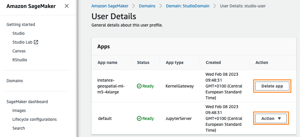
From the User profiles list, select studio-user, and then delete all the apps listed under Apps by choosing Delete app.
To delete the JupyterServer, choose Action, then choose Delete.
Wait until the Status changes to Deleted.
Delete the CloudFormation Stack
If you used an existing SageMaker Studio domain, you can skip the rest of the steps, and proceed directly to the conclusion section.
If you ran the CloudFormation template to create a new SageMaker Studio domain, continue with the following step to delete the domain, user, and the resources created by the CloudFormation template.
1. Delete the CloudFormation stack
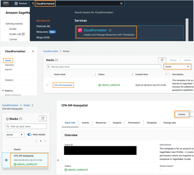
Navigate to the CloudFormation console.
In the CloudFormation pane, choose Stacks. From the status dropdown list, select Active. Under Stack name, choose CFN-SM-Geospatial to open the stack details page.
On CFN-SM-Geospatial stack details page, choose Delete to delete the stack along with the resources it created.
Conclusion
Congratulations! You have finished the tutorial on how to assess wildfire damage with Amazon SageMaker geospatial capabilities.
In this tutorial, you used Amazon SageMaker geospatial capabilities to create and visualize an Earth Observation Job, exported its data to S3 and performed further computations on the data.
Did you find what you were looking for today?
Let us know so we can improve the quality of the content on our pages
