Automate your Amazon Redshift performance tuning with automatic table optimization

Amazon Redshift is a cloud data warehouse database that provides fast, consistent performance running complex analytical queries on huge datasets scaling into petabytes and even exabytes with Amazon Redshift Spectrum. Although Amazon Redshift has excellent query performance out of the box, with up to three times better price performance than other cloud data warehouses, you can further improve its performance by physically tuning tables in a data model. You do so by sorting table rows and rearranging rows across a cluster’s nodes. In Amazon Redshift, you implement this by setting sort and distribution key table attributes.

In the past, setting sort and distribution keys was an involved manual process that required a skilled resource to analyze a cluster’s workload and choose and implement the right keys for every table in the data model. More recently, Amazon Redshift Advisor provided suggestions, but these still had to be manually implemented. At AWS re:Invent 2020, Amazon Redshift announced a new feature to automate this process: automatic table optimization (ATO). ATO automatically monitors a cluster’s workload and table metadata, runs artificial intelligence algorithms over the observations, and implements sort and distribution keys online in the background, without requiring any manual intervention, and without interrupting any running queries.

In this post, I explain what sort and distribution keys are and how they improve query performance. I also explain how ATO works and how to enable and disable it. Then I outline the steps to set up and run a test of ATO on the Cloud DW benchmark derived from TPC-H using a 30 TB dataset. Finally, I present the results of a test that show ATO improved performance on this benchmark, without requiring any manual tuning.

Distribution and sort keys

In this section, I give a high-level overview of distribution and sort keys, then I explain how they’re automatically set by ATO.

Distribution keys

Amazon Redshift has a massively parallel processing (MPP) architecture, where data is distributed across multiple compute nodes (see the following diagram). This allows Amazon Redshift to run queries against each compute node in parallel, dramatically increasing query performance.

To achieve the best possible query performance, data needs to be distributed across the compute nodes in a way that is optimal to the specific workload that is being run on the cluster. For example, the optimal way to distribute data for tables that are commonly joined is to store rows with matching join keys on the same nodes. This enables Amazon Redshift to join the rows locally on each node without having to move data around the nodes. Data distribution also affects the performance of GROUP BY operations.

In Amazon Redshift, the data distribution pattern is determined by two physical table settings: distribution style (DISTSTYLE) and distribution key (DISTKEY).

Amazon Redshift has three distribution styles:

• All – A copy of the entire table is replicated to every node
• Even – The data in the table is spread evenly across the nodes in a cluster in a round-robin distribution
• Key – The data is distributed across the nodes by the values in the column defined as the DISTKEY

If a table’s distribution style is key, then a single column in the table can be set as the DISTKEY.

Sort keys

Sort keys determine how rows are physically sorted in a table. Having table rows sorted improves the performance of queries with range-bound filters. Amazon Redshift stores the minimum and maximum values of each of its data blocks in metadata. When a query filters on a column (or multiple columns), the execution engine can use the metadata to skip blocks that are out of the filter’s range. For example, if a table has a sort key on the column created_date and a query has a filter WHERE created_date BETWEEN '2020-02-01' AND '2020-02-02', the execution engine can identify which blocks don’t contain data for February 1 and 2 given their metadata. The execution engine can then skip over these blocks, reducing the amount of data read and the number of rows that need to be materialized and processed, which improves the query performance.

Sort keys can be set on a single column in a table, or multiple columns (known as a compound sort key). They can also be interleaved.

Manually set distribution and sort keys

When you create a table in Amazon Redshift, you can manually set the distribution style and key, and the sort key in the CREATE TABLE DDL.

The following code shows two simplified example DDL statements for creating a dimension and fact table in a typical star schema model that manually set distribution and sort keys:

CREATE TABLE customer_dim (
   customer_key INT  
  ,customer_id INT
  ,first_name VARCHAR(100)
  ,last_name VARCHAR(100)
  ,join_date DATE) 
DISTKEY ( customer_key );

CREATE TABLE sale_fact (
   date_key DATE SORTKEY
  ,customer_key INT  
  ,product_key INT
  ,sale_amount DECIMAL(7,2))
DISTKEY ( customer_key );

Both tables have the customer_key column set as the distribution key (DISTKEY). When rows are inserted into these tables, Amazon Redshift distributes them across the cluster based on the values of the customer_key column. For example, all rows with a customer_key of 100 are moved to the same node, and likewise all rows with a customer_key of 101 are also moved to the same node (this may not be the same node as the key of 100), and so on for every row in the table.

In the sale_fact table, the date_key column has been set as the sort key (SORTKEY). When rows are inserted into this table, they’re physically sorted on the disk in the order of dates in the date_key column.

After data has been loaded into the tables, we can use the svv_table_info system view to see what keys have been set:

INSERT INTO customer_dim (customer_key, customer_id, first_name, last_name, join_date)
VALUES (100, 1001, 'John', 'Smith', SYSDATE);

INSERT INTO sale_fact (date_key, customer_key, product_key, sale_amount)
VALUES (SYSDATE, 100, 203, 98.76);

SELECT ti."table"      
      ,ti.diststyle      
      ,ti.sortkey1
FROM svv_table_info ti
WHERE ti.database = 'dev'
AND ti.schema = 'public'
AND ti."table" IN ('customer_dim', 'sale_fact')
ORDER BY 1;

The following table shows our results.

The sort key for customer_dim has been set to AUTO(SORTKEY), which I explain in the next section.

Now, if we populate these tables and run a business analytics query on them, like the following simplified query, we can see how the distribution and sort keys improve the performance of the query:

SELECT cd.customer_id      
     ,SUM(sf.sale_amount) AS sale_amount
FROM sale_fact sf
INNER JOIN customer_dim cd   
   ON sf.customer_key = cd.customer_key
WHERE sf.date_key BETWEEN '2021-03-01' AND '2021-03-07'
GROUP BY cd.customer_id;

The customer_dim table is joined to the sale_fact table on the customer_key column. Because both the table’s rows are distributed on the customer_key column, this means the related rows (such as customer_key of 100) are co-located on the same node, so when Amazon Redshift runs the query on this node, it doesn’t need to move related rows across the cluster from other nodes (a process known as redistribution) for the join. Also, there is a range bound filter on the date_key column (WHERE sf.date_key BETWEEN '2021-03-01' AND '2021-03-07'). Because there is a sort key on this column, the Amazon Redshift execution engine can more efficiently skip blocks that are out of the filter’s range.

Automatically set distribution and sort keys

Amazon Redshift ATO is enabled by default. When you create a table and don’t explicitly set distribution or sort keys in the CREATE TABLE DDL (as in the previous example), the following happens:

• The distribution style is set to AUTO(ALL) for small tables and AUTO(EVEN) for large tables.
• The sort key is set to AUTO(SORTKEY). This means no sort key is currently set on the table.

The AUTO keyword indicates the style and key are being managed by ATO.

For example, we can create a table with no keys explicitly defined:

CREATE TABLE customer_dim (
   customer_key INT  
  ,customer_id INT  
  ,first_name VARCHAR(100)
  ,last_name VARCHAR(100)
  ,join_date DATE);

Then we insert some data and look at the results from svv_table_info:

INSERT INTO customer_dim (customer_key, customer_id, first_name, last_name, join_date)
VALUES (100, 1001, 'John', 'Smith', SYSDATE);

SELECT ti."table"      
      ,ti.diststyle      
      ,ti.sortkey1
FROM svv_table_info ti
WHERE ti.database = 'dev'
AND ti.schema = 'public'
AND ti."table" IN ('customer_dim', 'sale_fact')
ORDER BY 1;

The following table shows our results.

The distribution and sort key are being managed by ATO, and the distribution style has already been set to ALL.

ATO now monitors queries that access customer_dim and analyzes the table’s metadata, and makes several observations. An example of an observation is the amount of data that is moved across nodes to perform a join, or the number of times a column was used in a range-scan filter that would have benefited from sorted data.

ATO then analyzes the observations using AI algorithms to determine if the introduction or change of a distribution or sort key will improve the workload’s performance.

For distribution keys, Amazon Redshift constructs a graph representation of the SQL join history, and uses this graph to calculate the optimal table distribution to reduce data transfer across nodes when joining tables (see the following diagram). You can find more details of this process in the scientific paper Fast and Effective Distribution-Key Recommendation for Amazon Redshift.

For sort keys, a table’s queries are monitored for columns that are frequently used in filter and join predicates. A column is then chosen based on the frequency and selectivity of those predicates.

When an optimal configuration is found, ATO implements the new keys in the background, redistributing rows across the cluster and sorting tables. For sort keys, another Amazon Redshift feature, automatic table sort, handles physically sorting the rows in the table, and maintains the sort order over time.

This whole process, from monitoring to implementation, completes in hours to days, depending on the number of queries that are run.

Convert existing tables to automatic optimization

You can enable ATO on existing tables by setting the distribution style and sort key to AUTO with the ALTER TABLE statement. For example:

ALTER TABLE customer_dim ALTER DISTSTYLE AUTO;

ALTER TABLE customer_dim ALTER SORTKEY AUTO;

If the table has existing sort and/or distribution keys that were explicitly set, then currently they will be preserved and won’t be changed by ATO.

Disable automatic table optimization

To disable ATO on a table, you can explicitly set a distribution style or key. For example:

ALTER TABLE customer_dim ALTER DISTSTYLE ALL;

ALTER TABLE customer_dim ALTER DISTSTYLE EVEN;

ALTER TABLE customer_dim ALTER DISTKEY customer_id;

You can then explicitly set a sort key or set the sort key to NONE:

ALTER TABLE customer_dim ALTER SORTKEY (join_date);

ALTER TABLE customer_dim ALTER SORTKEY NONE;

Performance test and results

Cloud DW benchmark derived from TPC-H

TPC-H is an industry standard benchmark designed to measure ad hoc query performance for business analytics workloads. It consists of 8 tables and 22 queries designed to simulate a real-world decision support system. For full details of TPC-H, see TPC BENCHMARK H.

The following diagram shows the eight tables in the TPC-H data model.

The Cloud DW Benchmark is derived from TPC-H and uses the same set of tables, queries, and a 30 TB dataset in Amazon Simple Storage Service (Amazon S3), which was generated using the official TPC-H data generator. This provides an easy way to set up and run the test on your own Amazon Redshift cluster.

Because the Cloud DW benchmark is derived from the TPC-H benchmark, it isn’t comparable to published TPC-H results, because the results of our tests don’t fully comply with the specification. This post uses the Cloud DW benchmark.

Set up the test

The following steps outline how to set up the TPC-H tables on an Amazon Redshift cluster, import the data, and set up the Amazon Redshift scheduler to run the queries.

Create an Amazon Redshift cluster

We recommend running this test on a five-node ra3.16xlarge cluster. You can run the test on a smaller cluster, but the query run times will be slower, and you may need to adjust the frequency the test queries are run at, such as every 4 hours instead of every 3 hours. For more information about creating a cluster, see Step 2: Create a sample Amazon Redshift cluster. We also recommend creating the cluster in the us-east-1 Region to reduce the amount of time required to copy the test data.

Set up permissions

For this test, you require permissions to run the COPY command on Amazon Redshift to load the test data, and permissions on the Amazon Redshift scheduler to run the test queries.

AWS Identity and Access Management (IAM) roles grant permissions to AWS services. The following steps describe how to create and set up two separate roles with the required permissions.

The RedshiftCopyRole role grants Amazon Redshift read-only access on Amazon S3 so it can copy the test data.

1. On the IAM console, on the Role page, create a new role called RedshiftCopyRole using Redshift – Customizable as the trusted entity use case.
2. Attach the policyamazonS3ReadOnlyAccess.

The RedshiftATOTestingRole role grants the required permissions for setting up and running the Amazon Redshift scheduler.

3. On the IAM console, create a new role called RedshiftATOTestingRole using Redshift – Customizable as the trusted entity use case.
4. Attach the following policies:
   1. amazonRedshiftDataFullAccess
   2. amazonEventBridgeFullAccess
5. Create a new policy called RedshiftTempCredPolicy with the following JSON and attach it to the role. Replace {DB_USER_NAME} with the name of the Amazon Redshift database user that runs the query.

{
	"Version": "2012-10-17",
	"Statement": [
		{
			"Sid": "UseTemporaryCredentials",
			"Effect": "Allow",
			"Action": "redshift:GetClusterCredentials",
			"Resource": [
			"arn:aws:redshift:*:*:dbuser:*/{DB_USER_NAME}"
			]
		}
	]
}

This policy assigns temporary credentials to allow the scheduler to log in to Amazon Redshift.

6. Check the role has the policies RedshiftTempCredPolicy, amazonEventBridgeFullAccess, and amazonEventBridgeFullAccess attached.
   
7. Now edit the role’s trust relationships and add the following policy:

   {
      "Sid": "S1",
      "Effect": "Allow",
      "Principal": {
        "Service": "events.amazonaws.com"
      },
      "Action": "sts:AssumeRole"
    }

The role should now have the trusted entities as shown in the following screenshot.

Now you can attach the role to your cluster.

8. On the Amazon Redshift console, choose your test cluster.
9. On the Properties tab, choose Cluster permissions.
10. Select Manage IAM roles and attach RedshiftCopyRole.

It may take a few minutes for the roles to be applied.

The IAM user that sets up and runs the Amazon Redshift scheduler also needs to have the right permissions. The following steps describe how to assign the required permissions to the user.

11. On the IAM console, on the Users page, choose the user to define the schedule.
12. Attach the policy amazonEventBridgeFullAccess directly to the user.
13. Create a new policy called AssumeATOTestingRolePolicy with the following JSON and attach it to the user. Replace {AWS ACCOUNT_NUMBER} with your AWS account number.

{
	"Version": "2012-10-17",
	"Statement": [
		{
		"Sid": "AssumeIAMRole",
		"Effect": "Allow",
		"Action": "sts:AssumeRole",
		"Resource": "arn:aws:iam::{AWS ACCOUNT_NUMBER}:role/RedshiftATOTestingRole"
		}
	]
}

This policy allows the user to assume the role RedshiftATOTestingRole, which has required permissions for the scheduler.

The user should now have the AssumeATOTestingRolePolicy and amazonEventBridgeFullAccess policies directly attached.

Create the database tables and copy the test data

The following script is an untuned version of the TPC-H ddl.sql file that creates all required tables for the test and loads them with the COPY command. To untune the tables, all the sort and distribution keys have been removed. The original tuned version is available on the amazon-redshift-utils GitHub repo.

Copy the script into your Amazon Redshift SQL client of choice, replace the <AWS ACCOUNT_NUMBER> string with your AWS account number, and run the script. On a five-node ra3.16xlarge cluster in the us-east-1 Region, the copy should take approximately 3 hours.

The script creates tables in the default schema public. For this test, I have created a database called tpch_30tb, which the script is run on.

ddl_untuned.sql

When the copy commands have finished, run the following queries to see the table’s physical settings:

SELECT ti."table"      
      ,ti.tbl_rows      
      ,ti.size      
      ,ti.diststyle      
      ,ti.sortkey1      
      ,ti.sortkey_num      
      ,ti.encoded
FROM svv_table_info ti
WHERE ti.database = 'tpch_30tb'
AND ti.schema = 'public'
ORDER BY ti.size;

The output of this query shows some optimizations have already been implemented by the COPY command. The smaller tables have the diststyle set to ALL (replicating all rows across all data nodes), and the larger tables are set to EVEN (a round-robin distribution of rows across the data nodes). Also, the encoding (compression) has been set for all the tables.

SELECT td.tablename      
      ,td."column"      
      ,td.encoding
FROM pg_table_def td
WHERE td.tablename = 'customer'
AND   td.schemaname = 'public';

This output shows the encoding type set for each column of the customer table. Because Amazon Redshift is a columnar database, the compression can be set differently for each column, as opposed to a row-based database, which can only set compression at the row level.

Schedule the test queries

The TPC-H benchmark uses a set of 22 queries that have a wide variation of complexity, amount of data scanned, answer set size, and elapsed time. For this test, the queries are run in serial from a single script file query0.sql. Because Query 11 (Q11) returns a large number of rows and the goal of this test was to measure execution time, this benchmark included a limit 1000 statement on the query to ensure the time being measured was predominantly execution time, rather than return time. This script is available on the amazon-redshift-utils GitHub repo under the src/BlogContent/ATO directory.

At the top of the script, enable_result_cache_for_session is set to off. This forces Amazon Redshift to rerun the queries on each test run, and not just return the query results from the results cache.

Use the following steps to schedule the test script:

1. Download query0.sql from GitHub.
2. Make sure the IAM user has been granted the necessary permissions (set in a previous step).
3. On the Amazon Redshift console, open the query editor.
4. If the current tab is blank, enter any text to enable the Schedule button.
5. Choose Schedule.
   
6. Under Scheduler permissions for IAM role, specify the IAM role you created in a previous step (RedshiftATOTestingRole).
7. For Cluster, choose your cluster.
8. Enter values for Database name and Database user.
   
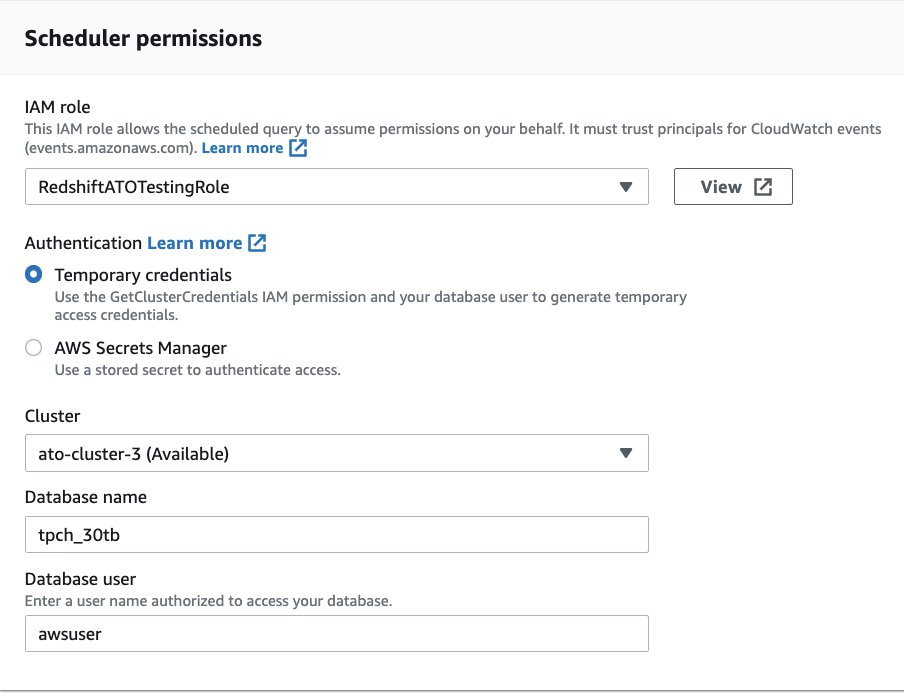
9. Under Query information, for Scheduled query name, enter tpch-30tb-test.
10. Choose Upload Query and choose the query0.sql file you downloaded in a previous step.
    
11. Under Scheduling options, change Repeat every: to 3 hours.

If you have a smaller cluster, each test run requires more time. To determine the amount of time needed, run query0.sql once to determine the runtime and add an hour for ATO to perform its processing.

12. For Repeat on:, select Everyday.
    
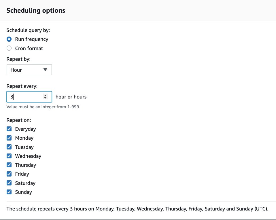
13. Choose Save changes.

The test queries are now set to run in the background at the given schedule. Leave the schedule running for approximately 48 hours to run a full test.

Check the table changes

Amazon Redshift automatically monitors the workload on the cluster and uses AI algorithms to calculate the optimal sort and distribution keys. Then ATO implements the table changes online, without disrupting running queries.

The following queries show the changes ATO has made and when they were made:

SELECT ti."table"      
      ,ti.diststyle      
      ,ti.sortkey1
FROM svv_table_info ti
WHERE ti.database = 'tpch_30tb'
AND ti.schema = 'public'
ORDER BY ti."table";

The following table shows our output.

Now we can see all the distribution and sort keys that have been set by ATO.

svl_auto_worker_action is an Amazon Redshift system view that allows us to see a log of the changes made by ATO:

SELECT st."table"      
      ,wa.type      
      ,wa.status      
      ,wa.eventtime         
      ,wa.previous_state
FROM svl_auto_worker_action wa
INNER JOIN svv_table_info st   
   ON wa.table_id = st.table_id
ORDER BY eventtime;

Data in the following table has been abbreviated to save space.

We can see when each change was implemented by ATO. First, a DISTKEY was added to the supplier table at 4:17 AM on June 25. Because this table is relatively small (300 million rows), ATO was able to apply the DISTKEY in one step.

Next, ATO started implementing a DISTKEY on the part table at 4:20 AM. For DISTKEY changes on large tables (part has 6 billion rows), ATO creates a copy of the source table in the background (a shadow table) and then copies data from the source table into the shadow table, redistributing the data according to the new DISTKEY. This process is done in batches known as checkpoints. After all the data has been copied, the metadata is updated, swapping the shadow table with the source table. There were seven checkpoints for part, and the full conversion was completed at 4:24 AM.

Then from 4:27 AM on June 25 until 4:55 AM on June 26, distribution keys were implemented on orders, customer, and partsupp. The last DISTKEY was then implemented on largest table in the model lineitem (179 billion rows), finishing at 8:41 AM. Because this table was so large, there were 261 checkpoints.

Finally, sort keys on supplier, part, orders and lineitem were created at 4:17 PM on June 26.

View the test results

Now we look at the output of the test and see what impact ATO’s changes had on the overall performance.

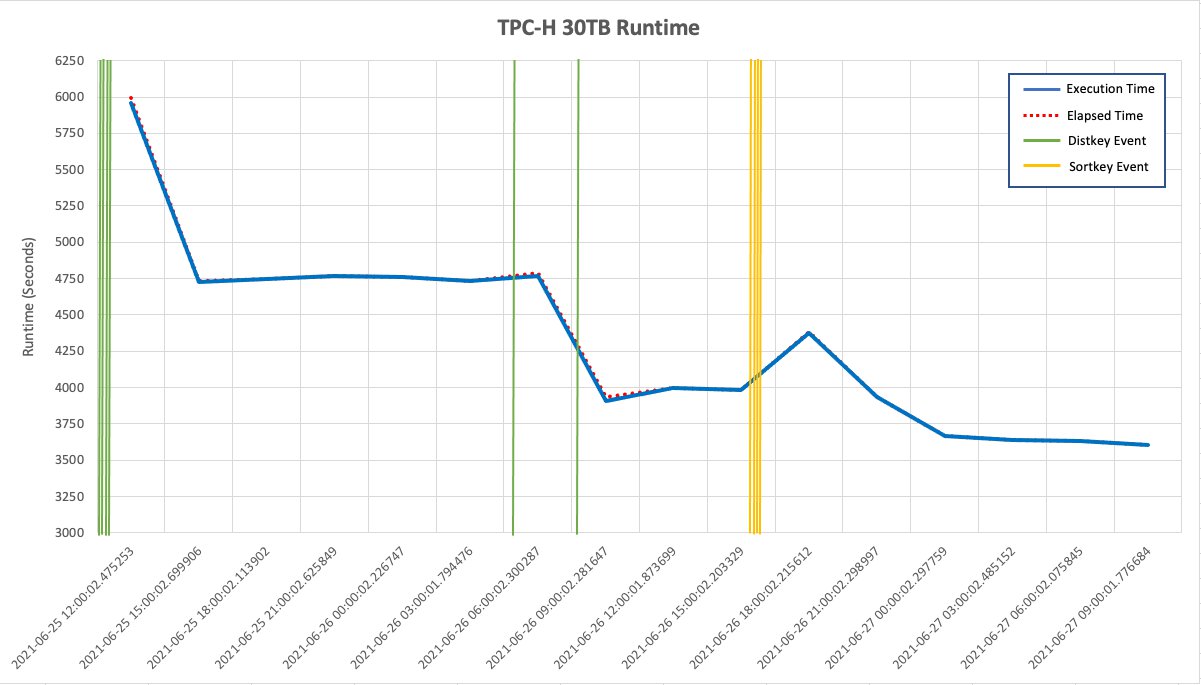
The following line graph shows the runtime of the query0.sql script over time. The vertical reference lines show when ATO changed a DISTKEY or SORTKEY. The first distribution keys were created before the test had actually started. This is because ATO was able to use table properties such as constraints to determine appropriate distribution keys. Over time, ATO may change these distribution keys based on workload observations.

The rest of the distribution keys were then added, and lastly the sort keys, reducing the runtime from approximately 4,750 seconds to 3,597.

The data for this graph is taken from the following query:

SELECT q.pid     
      ,COUNT(DISTINCT q.query) num_queries     
      ,MIN(q.starttime) starttime     
      ,MAX(q.endtime) endtime     
      ,DATEDIFF(SECOND, MIN(q.starttime), MAX(q.endtime)) elapsed_sec     
      ,SUM(DATEDIFF(SECOND, c.starttime, c.endtime)) compile_time     
      ,DATEDIFF(SECOND, MIN(q.starttime), MAX(q.endtime)) - SUM(DATEDIFF(SECOND, c.starttime, c.endtime)) exec_time
FROM stl_query q
INNER JOIN svl_compile c   
   ON q.query = c.query
WHERE q.userid > 1  
AND q.label LIKE 'RSPERF TPC-H%'
GROUP BY q.pid
ORDER BY starttime ASC;

The following table shows our results.

We take a baseline measurement of the runtime on the third run, which ensures any additional compile time is excluded from the test. When we look at the test runs from midnight on June 26 (after ATO had made its changes), we can see the performance improvement.

Clean up

After you have viewed the test results and ATO changes, be sure to decommission your cluster to avoid having to pay for unused resources. Also, delete the IAM policy RedshiftTempCredPolicy and the IAM roles RedshiftCopyRole and RedshiftATOTestingRole.

Cloud DW benchmark derived from TPC-H 3 TB results

We ran the same test using the 3 TB version of the Cloud DW benchmark derived from TPC-H. It ran on a 10-node ra3.4xlarge cluster with query0.sql run every 30 minutes. The results of the test showed ATO achieved a significant increase in performance of up to 25%.

Summary

With automatic table optimization, Amazon Redshift has further increased its automation capabilities to cover query performance tuning in addition to administration tasks.

In this post, I explained how distribution and sort keys improve performance and how they’re automatically set by ATO. I showed how ATO increased performance by up to 24% on a 30 TB industry-standard benchmark with no manual tuning required. I also outlined the steps for setting up the same test yourself.

I encourage you to try out ATO by setting up an Amazon Redshift cluster and running the test, or enabling ATO on existing and new tables on your current cluster and monitoring the results.

About the Author

Adam Gatt is a Senior Specialist Solution Architect for Analytics at AWS. He has over 20 years of experience in data and data warehousing and helps customers build robust, scalable and high-performance analytics solutions in the cloud.