Optimizing correlated subqueries in Amazon Aurora PostgreSQL

Correlated subqueries can cause performance challenges in Amazon Aurora PostgreSQL-Compatible Edition, often causing applications to experience reduced performance as data volumes grow. In this post, we explore the advanced optimization configurations available in Aurora PostgreSQL that can transform these performance challenges into efficient operations without requiring you to modify a single line of SQL code. The configurations we are going to explore are the subquery transformation and the subquery cache optimizations.

If you’re experiencing performance impacts due to correlated subqueries or planning a database migration where rewriting a query using correlated subquery to a different form isn’t feasible, the optimization capabilities of Aurora PostgreSQL could deliver the performance improvement you need.

Understanding correlated subqueries

A correlated subquery is a nested query that references columns from its outer query, creating a dependency that requires the inner query to execute once for each row processed of the outer query. This relationship is what makes them both powerful and potentially problematic for performance.

Anatomy of a correlated subquery

The following diagram shows a correlated subquery that finds the maximum order amount for each customer by looking up their orders in a separate table. For each customer row in the main query, the subquery executes once to find that specific customer’s highest order total using the matching customer_id from the orders table.

-- OUTER QUERY: The main query that selects from the customers table
SELECT customer_name, 
( 
	-- INNER QUERY: Correlated subquery that finds the max order for each customer
	SELECT MAX(o.total_amount) 
	FROM orders o 
	WHERE o.customer_id = c.customer_id 
) AS max_order_amount 
FROM customers c; -- OUTER QUERY: customers table with alias 'c'

Key components:

• Outer query: Processes the main dataset (customers table)
• Inner query: The subquery that depends on outer query values
• Correlation condition: o.customer_id = c.customer_id links the queries
• Correlated column: c.customer_id from the outer query used in the inner query

The performance challenge

Traditional execution of correlated subqueries follows this pattern:

1. Fetch one row from the outer query
2. Execute the subquery with correlated values fetched from step 1
3. Return the subquery result
4. Repeat for the next outer row

For 10,000 customers with 500 orders each, this would imply 10,000 separate subquery executions, resulting in sub-optimal performance for the query.

Aurora PostgreSQL provides two powerful methods to overcome the performance challenges of correlated subqueries: subquery transformation optimization and subquery cache optimization.

Subquery transformation

The subquery transformation optimization automatically converts correlated subqueries into efficient join-based execution plans. Instead of running the same subquery repeatedly for each row in your outer table, this optimization runs the subquery just once and stores the results in a hash lookup table. The outer query then simply looks up the answers it needs from the hash table, which is much faster than recalculating the same thing repeatedly.

The subquery transformation feature delivers the greatest reduction in query execution time in several key scenarios. When your outer query is expected to return large result sets of more than 1,000 rows, the transformation can significantly improve performance. The feature excels with expensive subqueries that include aggregations, complex joins, and sorting operations within the subquery itself. It proves particularly valuable when indexes are missing on correlation columns, because the transformation eliminates the need for these indexes. Migration scenarios where rewriting queries isn’t feasible represent another ideal use case; you can use subquery transformation to improve performance without modifying existing SQL code. A best-case scenario for the subquery transformation optimization occurs when the table is large and has missing indexes and the subquery result uses aggregation functions.

How to enable subquery transformation

Aurora PostgreSQL can automatically transform eligible correlated subqueries into efficient join operations. This can be enabled at either the session or parameter group level.

-- Enable the transformation feature at the session level
SET apg_enable_correlated_scalar_transform = on;

-- Enable it at the parameter group level
aws rds modify-db-cluster-parameter-group \
--db-cluster-parameter-group-name mydbclusterparametergroup \
--parameters "ParameterName=apg_enable_correlated_scalar_transform,ParameterValue=1,ApplyMethod=immediate"

-- Verify it is enabled at the psql prompt 
SHOW apg_enable_correlated_scalar_transform

Limitations and scope

The transformation applies only when the following conditions are met:

• Correlated columns appear only in the subquery WHERE clause
• Subquery WHERE conditions use AND operators exclusively
• The subquery must return a scalar value using aggregate functions like: MAX, MIN, AVG, COUNT, or SUM.
• No LIMIT, OFFSET, or ORDER BY operators can be present in the subquery
• There are no indexes present on the outer query or subquery join columns

The following are examples of queries that would not be optimized by subquery transformation based on these limitations:

A correlated field in a SELECT clause:

SELECT customer_name, 
(SELECT MAX(o.total_amount) * c.discount_factor -- unsupported
FROM orders o WHERE o.customer_id = c.customer_id)
FROM customers c;

OR conditions in a WHERE clause:

SELECT customer_name, 
(SELECT MAX(o.total_amount)
FROM orders o 
WHERE o.customer_id = c.customer_id OR o.status = 'active') -- unsupported
FROM customers c;

A LIMIT in the subquery:

SELECT customer_name, 
(SELECT AVG(o.total_amount)
FROM orders o WHERE o.customer_id = c.customer_id
LIMIT 5) -- unsupported 
FROM customers c;

The subquery cache

The subquery cache optimization stores and reuses subquery results for repeated correlation values, reducing computational overhead and improving performance when the same subquery conditions are evaluated multiple times. The ideal scenario for enabling the subquery cache is when you have high correlation value repetition (many rows with the same attributes), expensive subquery computations, queries ineligible for plan transform, and when the cached result is finite. A perfect example scenario occurs when the subquery condition is too complicated, so the subquery transform won’t work for the query, and the cache hit rate is more than 30%, which indicates there are repeated rows in the outer table.

The subquery cache optimization adds a PostgreSQL Memoize node, a caching layer between a nested loop and its inner subquery, storing results to avoid redundant computations. Instead of executing the subquery for every customer row, the Memoize node:

• Caches results based on the customer_id (cache key).
• Reuses cached results when the same customer_id appears again.
• Reduces redundant computations by storing previously calculated max (total_amount) values.

How to enable subquery caching

Subquery caching complements transformation by storing and reusing subquery results. It can be enabled in two ways.

You can enable subquery caching at the session level:

SET apg_enable_subquery_cache = on;

You can also enable in your cluster parameter group, using the following dynamic parameter:

aws rds modify-db-cluster-parameter-group \
--db-cluster-parameter-group-name mydbclusterparametergroup \
--parameters "ParameterName=apg_enable_subquery_cache,ParameterValue=1,ApplyMethod=immediate"

Finally, you can check the change has been applied:

SHOW apg_enable_subquery_cache;

Limitations and scope

The following are subquery types that are can be used in the subquery cache:

• Scalar subqueries with correlation
• Deterministic functions only
• Hashable correlation column types

The operators IN, ANY, ALL cannot be used with statements in the subquery cache.

When to use subquery transform or subquery cache

The subquery cache can be enabled independently of subquery transformation, which means you can use subquery caching as a standalone performance enhancement or in combination with subquery transformation for maximum optimization. Use subquery transformation by itself when you have large datasets with minimal repeated values and your subqueries meet the strict requirements, because it can significantly reduce execution time by converting nested loops into efficient joins. Use the subquery cache when your queries have complex conditions that prevent transformation but contain many repeated correlation values, allowing the cache to store and reuse results even when transformation isn’t possible.

Where subqueries meet the requirements for both subquery transformation and caching because of repeated correlation values, then you will get maximum benefit by using both optimizations:

-- Enable both optimizations
SET apg_enable_correlated_scalar_transform = on;
SET apg_enable_subquery_cache = on;

In such cases, the optimizer will do the transform first and subsequently the subquery cache will be used to build the query plan.

Subquery optimizations in action

Let’s look at how to use these two optimizations in practice. For subquery transformation, we will measure impact in query execution time before and after optimization. For subquery cache, we will measure impact in cache hit ratio (CHR).

Subquery transformation impact

To review the impact of subquery transformation, we start by generating test data. The following data preparation SQL statements create two tables, the first called inner_table with three columns (id, a, and b) and populates it with 10,000 rows of data where column a cycles through values 1–100 and column b contains random numbers. The code then fills the second outer_table with 50,000 rows split between repeated values (1–100) and unique values (101–25100), followed by gathering statistics on both tables.

-- We create tables
CREATE TABLE outer_table (
id SERIAL PRIMARY KEY,
a INT,
b INT
);
CREATE TABLE inner_table (
id SERIAL PRIMARY KEY,
a INT,
b INT
);
-- Insert data into inner table with some randomness
INSERT INTO inner_table (a, b)
SELECT 
1 + mod(generate_series - 1, 100), -- 100 rows per 'a' value
floor(random() * 1000)::int
FROM generate_series(1, 10000);

-- Insert data into outer table
-- First 25K rows with values 1-100 (repeated values)
INSERT INTO outer_table (a, b)
SELECT 
1 + mod(generate_series - 1, 100),
floor(random() * 1000)::int
FROM generate_series(1, 25000);

-- Next 25K rows with values 101-25100 (unique values)
INSERT INTO outer_table (a, b)
SELECT 
generate_series + 100,
floor(random() * 1000)::int
FROM generate_series(1, 25000);

INSERT INTO outer_table (a, b)
SELECT 
generate_series + 100, -- Unique a values starting from 101
floor(random() * 1000)::int -- Random b values
FROM generate_series(1, 25000);

-- Gather updated statistics
ANALYZE outer_table;
ANALYZE inner_table;

An index isn’t needed in this example, because correlated subquery transformation works best without indexes. This is because subquery transformations can remove the need for indexes by converting multiple table scans into a single table scan, reducing query complexity and avoiding the storage overhead and Data Manipulation Language (DML) latency penalties associated with maintaining indexes.

Before enabling the transformation:

explain analyze SELECT outer_table.a, outer_table.b,
(SELECT AVG(inner_table.b) FROM inner_table
WHERE inner_table.a = outer_table.a) FROM outer_table;
QUERY PLAN
----------------------------------------------------------------------------------------------------------------------------
Seq Scan on outer_table (cost=0.00..9013896.00 rows=50000 width=40) (actual time=0.894..41856.498 rows=50000 loops=1)
SubPlan 1
-> Aggregate (cost=180.25..180.26 rows=1 width=32) (actual time=0.836..0.836 rows=1 loops=50000)
-> Seq Scan on inner_table (cost=0.00..180.00 rows=100 width=4) (actual time=0.419..0.831 rows=50 loops=50000)
Filter: (a = outer_table.a)
Rows Removed by Filter: 9950
Planning Time: 0.083 ms
Execution Time: 41860.809 ms
(8 rows)

After enabling the transformation:

Sections indicating that a hash lookup table is being used instead of repeated subquery executions for every row in the outer table are highlighted in bold.

explain analyze SELECT outer_table.a, outer_table.b,
(SELECT AVG(inner_table.b) FROM inner_table
WHERE inner_table.a = outer_table.a) FROM outer_table;
QUERY PLAN
---------------------------------------------------------------------------------------------------------------------------------
Hash Left Join (cost=207.50..1109.78 rows=50000 width=40) (actual time=3.008..18.671 rows=50000 loops=1)
Hash Cond: (outer_table.a = inner_table.a)
-> Seq Scan on outer_table (cost=0.00..771.00 rows=50000 width=8) (actual time=0.010..5.132 rows=50000 loops=1)
-> Hash (cost=206.25..206.25 rows=100 width=36) (actual time=2.992..2.994 rows=100 loops=1)
Buckets: 1024 Batches: 1 Memory Usage: 13kB
-> HashAggregate (cost=205.00..206.25 rows=100 width=36) (actual time=2.930..2.965 rows=100 loops=1)
Group Key: inner_table.a
Batches: 1 Memory Usage: 32kB
-> Seq Scan on inner_table (cost=0.00..155.00 rows=10000 width=8) (actual time=0.008..0.895 rows=10000 loops=1)
Planning Time: 0.156 ms
Execution Time: 20.807 ms
(11 rows)

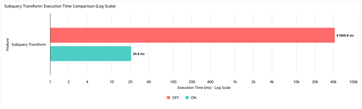
The following graph shows the execution time (in milliseconds) in a test case with an inner table of 10,000 rows and an outer table of 75,000 rows. By using the subquery transform, the query execution time is reduced by 99.95% compared to not using the feature, from 41seconds down to 20.8 milliseconds. The percentage improvement realized is data-dependent, but this example demonstrates the scale of improvement that can be achieved.

Subquery cache impact

Just like reviewing the impact of subquery transformation, the first step to review the impact of using a subquery cache is to generate test data. The following SQL code creates two tables (outer_table and inner_table) with identical structures (id, a, bcolumns) and populates inner_table with 10,000 sequential rows while filling outer_table with 100,000 rows split between repeated values (1–100) in the first half and unique values (101–50100) in the second half. The script concludes by updating the database statistics for both tables using the ANALYZE command.

-- We drop the tables of the same name that existed before
DROP TABLE IF EXISTS outer_table;
DROP TABLE IF EXISTS inner_table;
-- We create the tables
CREATE TABLE outer_table (
id SERIAL PRIMARY KEY,
a INT,
b INT
);
CREATE TABLE inner_table (
id SERIAL PRIMARY KEY,
a INT,
b INT
);
-- Insert data into inner table with some randomness
INSERT INTO inner_table (a, b)
SELECT 
generate_series,
floor(random() * 1000)::int -- Random b values
FROM generate_series(1, 10000);
-- Insert data into outer table
-- First 50K rows with values 1-100 (repeated values)
INSERT INTO outer_table (a, b)
SELECT 
1 + mod(generate_series - 1, 100), -- a values cycle from 1-100
floor(random() * 1000)::int -- Random b values
FROM generate_series(1, 50000);
-- Next 50K rows with values 101-50100 (unique values)
INSERT INTO outer_table (a, b)
SELECT 
generate_series + 100, -- Unique a values starting from 101
floor(random() * 1000)::int -- Random b values
FROM generate_series(1, 50000);
-- Gather fresh statistics
ANALYZE outer_table;
ANALYZE inner_table;

An index isn’t needed because when indexes are present and usable, individual subquery executions might already be fast enough that caching provides diminishing returns.

Without the subquery cache:

postgres=> set apg_enable_subquery_cache= off;
SET
postgres=> explain analyze SELECT outer_table.a, outer_table.b, 
(SELECT AVG(inner_table.b) FROM inner_table 
WHERE inner_table.a = outer_table.a) FROM outer_table;
QUERY PLAN 
---------------------------------------------------------------------------------------------------------------------------
Seq Scan on outer_table (cost=0.00..18003041.00 rows=100000 width=40) (actual time=0.485..38607.351 rows=100000 loops=1)
SubPlan 1
-> Aggregate (cost=180.00..180.01 rows=1 width=32) (actual time=0.386..0.386 rows=1 loops=100000)
-> Seq Scan on inner_table (cost=0.00..180.00 rows=1 width=4) (actual time=0.175..0.385 rows=1 loops=100000)
Filter: (a = outer_table.a)
Rows Removed by Filter: 9999
Planning Time: 0.082 ms
Execution Time: 38611.835 ms
(8 rows)

With the subquery cache:
Highlighted in bold are the cache hits and misses showing a 49.9% CHR.

postgres=> explain analyze SELECT outer_table.a, outer_table.b, 
(SELECT AVG(inner_table.b) FROM inner_table 
WHERE inner_table.a = outer_table.a) FROM outer_table;
QUERY PLAN 
-------------------------------------------------------------------------------------------------------------------------------
Seq Scan on outer_table (cost=0.00..18004041.00 rows=100000 width=40) (actual time=0.472..19328.986 rows=100000 loops=1)
SubPlan 1
-> Memoize (cost=180.01..180.02 rows=1 width=32) (actual time=0.193..0.193 rows=1 loops=100000)
Cache Key: outer_table.a
Cache Mode: binary
Hits: 49900 Misses: 50100 Evictions: 0 Overflows: 0 Memory Usage: 4942kB
-> Aggregate (cost=180.00..180.01 rows=1 width=32) (actual time=0.384..0.385 rows=1 loops=50100)
-> Seq Scan on inner_table (cost=0.00..180.00 rows=1 width=4) (actual time=0.346..0.384 rows=0 loops=50100)
Filter: (a = outer_table.a)
Rows Removed by Filter: 10000
Planning Time: 0.083 ms
Execution Time: 19333.955 ms
(12 rows)

Understanding cache hit rate

The Cache Hit Rate determines cache effectiveness and is calculated like the following:

CHR = (Cache Hits) / (Total Cache Lookups)

From this output, we can determine our CHR in the preceding example to be 49.9%. In general, for the subquery cache, a CHR above 70% is considered excellent. A CHR rate above 30% is good, and below 30%, the cache can be disabled because of limited benefit.

This is because—unlike shared buffer CHRs, which can reasonably reach 90% or more because the same data pages are frequently accessed—a 70% CHR for subquery cache reflects realistic data distribution patterns where only a portion of users have duplicate correlation values. A 50% CHR means half the customers in the outer query have duplicate values (such as repeat purchases), which represents normal business scenarios, whereas expecting 90% would imply unrealistic data patterns where nearly all users have identical behaviours.

You can also set parameters related to the subquery cache to decide whether the cache gets used. For each cached subquery, after the number of cache misses defined by apg_subquery_cache_check_interval is exceeded, the system evaluates whether caching that particular subquery is beneficial by comparing the CHR against the apg_subquery_cache_hit_rate_threshold. If the CHR falls below this threshold, the subquery is removed from the cache. The following are the defaults for these parameters.

-- Configure cache behavior
SET apg_subquery_cache_check_interval = 500;
SET apg_subquery_cache_hit_rate_threshold = 0.3;

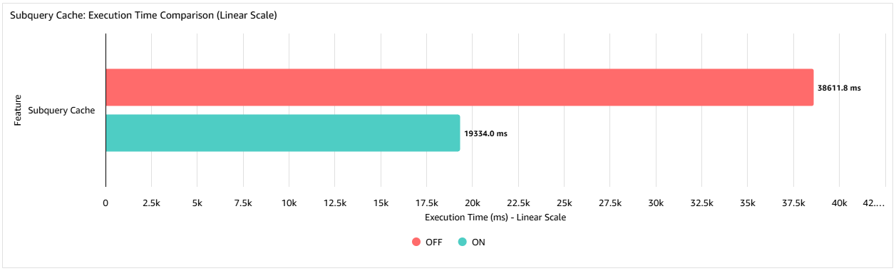
The following graph shows that in this example when using the subquery cache the query execution time is reduced to 50% of its original execution time. The improvement you achieve will vary from case to case. For example, the effectiveness of the cache will be influenced by the number of repeated rows in the outer query.

When to consider alternatives

Consider using the original PostgreSQL plan when you have excellent indexes already existing on correlation columns, queries execute infrequently, you have a small dataset for the outer query, or you’re dealing with complex subqueries with multiple correlation conditions. Consider manually rewriting the query when the plan is too complex to transform or when the cache hit rate is less than 30% in the subquery cache.

Conclusion

In this post, you have seen how the correlated subquery optimizations available in Aurora PostgreSQL can significantly improve performance through two complementary techniques: automatic subquery transformations and intelligent subquery caching. These features work together to tackle slow correlated queries without requiring code rewrites. Subquery transformation optimizes queries behind the scenes for significant speed improvements, while caching remembers results from expensive subqueries that repeatedly process similar data patterns. You can implement these optimizations incrementally, monitor their effects through Amazon CloudWatch, and test safely using the Amazon Aurora cloning and blue/green deployment features before production rollout, reducing the need to spend time rewriting complex queries and allowing Aurora to automatically handle the performance optimization heavy lifting.

To get started implementing these optimizations in your own environment, see Optimizing correlated subqueries in Aurora PostgreSQL and dive deeper into performance analysis techniques at this PostgreSQL page about reading EXPLAIN plans.

About the authors