AWS Spatial Computing Blog
Automate mining site compliance monitoring with AI-powered 3D scene understanding on AWS
Introduction
New techniques in 3D world modeling and AI-driven scene interpretation are unleashing a revolution in industries such as mining and construction. The global LiDAR market — valued at USD 2.74 billion in 2024 and projected to reach USD 4.71 billion by 2030 (9.5% CAGR) is generating unprecedented volumes of spatial sensor data. A single mobile LiDAR sensor can capture 600,000 points per second with sub-centimeter accuracy; a 100-day aerial survey of an active mine produces hundreds of millions of points per scan and terabytes of raw data in total. Processing these sequences to derive operational intelligence demands both cloud-scale compute and sophisticated AI processing pipelines.
A useful framework for understanding where a Computer Vision (CV) pipeline sits on the automation spectrum comes from our earlier post A maturity level framework for industrial inspection report automation (AWS Spatial Computing Blog, 2025). That framework defines four stages: Stage 0, basic 3D reconstruction; Stage 1, asset detection; Stage 2, differential scene understanding across successive captures; and Stage 3, fully automated AI-driven report generation requiring only lightweight human validation. Most deployments today are still at Stage 1. The pipeline in this post implements Stages 2 and 3 for open-pit mining.
This post is also a companion to End-to-end scalable vision intelligence pipeline using LiDAR 3D point clouds on AWS (AWS HPC Blog, 2026), which covers the cloud infrastructure layer — data ingestion, distributed processing on Amazon EC2, and cost-optimized storage on Amazon S3 — that underpins the analytical pipeline described here.
Open-pit mining operations generate some of the most dynamic physical changes on Earth. Over days and weeks, excavators carve millions of cubic meters of material, vegetation is cleared to expand work areas, water accumulates in low-lying zones, and heavy equipment traverses complex terrain — all simultaneously, across sites spanning several square kilometers. Figure 1 shows a photorealistic overview of a mining site reconstructed from a 100-day LiDAR temporal sequence, illustrating the scale and variety of change that operational monitoring must track.
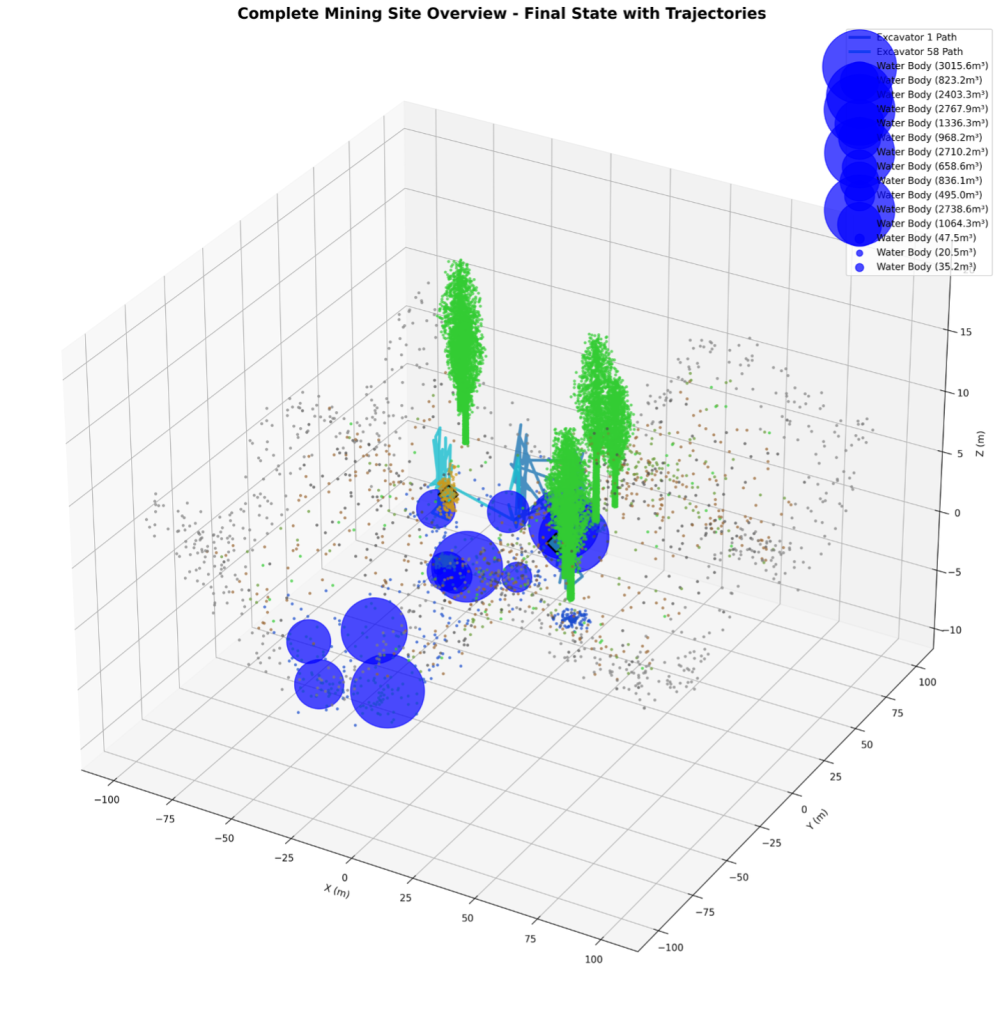
Figure 1. Complete mining site overview rendered from a 100-day LiDAR temporal sequence, showing excavation zones, vegetation boundaries, and water accumulation areas.
Manual monitoring is slow and error-prone. Environmental compliance demands precise, times-tamped evidence of what changed, where, and by how much. This post walks through a hybrid 4D temporal scene understanding pipeline that automatically monitors and documents site changes from raw LiDAR sequences — no manual labeling required.
The pipeline’s key innovation: repurposing 3D Gaussian Splatting — originally a rendering technique for novel-view synthesis — as a temporal segmentation engine. Extending Gaussian primitives into the time dimension (4D) gives the system smooth, continuous object tracking that classical frame-by-frame point cloud methods can’t match.
What you will learn
- How to build an end-to-end temporal 3D scene understanding pipeline for industrial environments
- How to fuse classical geometric methods with deep learning for robust object detection and tracking
- How 4D Gaussian Splatting enables smooth temporal modeling of dynamic point cloud scenes
- How to generate photorealistic, audit-ready evidence from LiDAR data for environmental compliance
- How to advance your inspection pipeline from Stage 2 to Stage 3 maturity
Prerequisites
To follow along with the code examples in this post, you need:
| Requirement | Details |
|---|---|
| Python | 3.9 or later |
| Core libraries | numpy, scipy, scikit-learn, matplotlib, torch, opencv |
| Point cloud I/O | laspy, open3d |
| Visualization | pillow, imageio |
| Skills | Familiarity with 3D point clouds and basic deep learning concepts |
| Data | LAS/LAZ format LiDAR frames with timestamps; the pipeline ships with a built-in synthetic data generator for evaluation without real survey data |
Install all dependencies with:
pip install -r requirements.txt
A novel use of Gaussian splatting for point cloud segmentation
3D Gaussian Splatting represents a scene as a collection of anisotropic Gaussian primitives — each with a 3D center, covariance matrix, opacity, and RGB color — composited via alpha blending from any camera angle. It was designed for one thing: photorealistic novel-view rendering. We use it for something different.
The same properties that make Gaussian primitives great renderers — continuity, differentiability, and spatially structured covariance — also make them ideal for encoding localized regions of a LiDAR point cloud. Instead of asking ‘what does this Gaussian look like from a given viewpoint?’, we ask ‘what object does it represent, and how does that object change over time?’ That shift unlocks a new application domain for the technique.
From 3D to 4D: the temporal extension
To enable temporal tracking, each Gaussian primitive is extended with time-domain parameters, forming a Gaussian4D object. The following table summarizes the three parameter groups that together encode both spatial appearance and temporal dynamics:
| Parameter Group | Parameters | Purpose |
|---|---|---|
| Spatial | center (x,y,z), covariance (3×3), opacity, RGB | Encodes object shape and appearance |
| Temporal | time_center, time_variance, velocity (vx,vy,vz) | Encodes object lifespan and motion |
| Deformation | Learnable MLP basis weights | Encodes non-rigid shape change over time |
A 4-layer neural Deformation Field MLP maps any (x, y, z, t) query to a 3D displacement vector, capturing non-rigid dynamics such as the gradual volumetric shrinkage of a tree canopy. DBSCAN clustering in the joint (x, y, z, t) space then extracts stable temporal tracklets — coherent object identity chains spanning dozens of frames — completing the segmentation task without manual labeling or class-specific supervision.
Pipeline architecture
The pipeline is organized into four layers. Raw LiDAR input flows through a dual-path scene understanding engine — a classical Point Transformer path for per-point semantic labels, and a 4D Gaussian path for temporal continuity — whose outputs are fused in a temporal analysis layer before reaching the intelligence layer that produces operational reports. The following table summarizes each layer and its components:
| Layer | Components |
|---|---|
| Input | LAS/LAZ LiDAR frames, Timestamps, Semantic pre-labels |
| Scene Understanding | Point Transformer segmentation, Sparse 3D convolutions, 4D Gaussian splatting |
| Temporal Analysis | Siamese change detection, Object tracklets, Deformation fields, DBSCAN clustering |
| Intelligence | Equipment tracking, Tree removal detection, Water volume estimation, Compliance reporting |
The two scene understanding paths are complementary by design. The classical path delivers semantic richness and noise robustness; the Gaussian path provides smooth object trajectories and memory-efficient continuous representations. The following table contrasts their respective strengths:
| Capability | Classical Path | Gaussian Path |
|---|---|---|
| Per-point semantic labels | Yes | No |
| Robust to sensor noise | Yes | Partial |
| Smooth object trajectories | Partial | Yes |
| Continuous deformation modeling | No | Yes |
| Memory-efficient representation | No | Yes |
The outputs of both paths are fused at the object-instance level: Point Transformer semantic labels define class identity, while Gaussian tracklets supply the continuous position and deformation history for each instance. Together, every tracked object carries both a semantic class (excavator, tree, water body) and a full 4D trajectory — the combination that enables the operational analytics described in the following section.
Core analytical capabilities
Equipment detection and pose tracking
Equipment points are clustered using a 12-meter search radius and validated against excavator dimensional constraints (3–15 m in XY, 2–8 m in Z). Pose is estimated via PCA eigendecomposition of the cluster covariance matrix, yielding roll, pitch, and yaw angles. Operational state is inferred per frame according to the following criteria:
| Operational State | Detection Criteria |
|---|---|
| Active | Point cloud shape consistent with boom extension |
| Digging | Large elevation delta detected in the proximity zone |
| Moving | Centroid displacement greater than 2 m between frames |
| Idle | No pose change exceeding 15 degrees, no proximal elevation change |
Figure 2 shows the reconstructed 100-day trajectory of two excavators tracked across four sequential work areas, with pose-oriented bounding boxes plotted at key waypoints. The system recorded a combined travel distance of 755.6 meters and flagged each significant orientation change exceeding 15 degrees as an operational event for the site log. Each plotted position includes the excavator’s estimated heading and color-coded operational state at that timestamp.
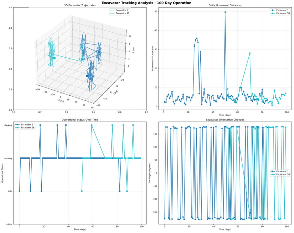
Figure 2. Excavator trajectory analysis: 100-day path reconstruction for two units, with pose-oriented bounding boxes at key positions and operational state color-coding (orange: active, yellow: idle, red: digging).
Tree removal detection and compliance evidence
Individual trees are clustered from vegetation points (semantic classes 2–4: low, medium, and high vegetation). Volume is computed using a four-method ensemble — ConvexHull, voxel counting (0.5 m resolution), cylindrical model, and bounding box — to maximize accuracy across tree types and point densities. Volume changes exceeding 10 m³ between consecutive frames trigger automatic removal classification, with each event assigned an alert level (low, medium, high, or critical) based on volume lost and proximity to protected zones.
For every confirmed removal event, the pipeline renders a photorealistic before/after comparison with full metadata — tree ID, timestamp, GPS coordinates, and volume lost — as audit-ready regulatory evidence. Figure 3 shows the detection dashboard summarizing 93 tree removal events documented over the 100-day reference period. The dashboard presents per-event confidence scores, volumetric measurements, and alert levels organized by severity, providing a complete audit trail suitable for environmental compliance submissions.
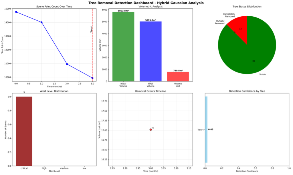
Figure 3. Tree removal detection dashboard: 93 events documented over 100 days, showing per-event confidence scores, vegetation volume lost (m³), and alert levels classified by severity.
Water body detection and volumetric tracking
Water accumulation is monitored using three parallel volume estimation methods: a 3D ConvexHull, a 0.5-meter voxel grid, and a cylindrical depth approximation. Surface area is derived from a 2D convex hull of the water point cluster, and depth is estimated from elevation differentials between the water surface and the underlying ground model. Three primary accumulation zones were tracked over the reference dataset, reaching a cumulative peak of 1,908,288 m³ at 20,399 m³ peak daily volume.
Oriented 3D bounding box visualization
All detected objects are represented with pose-aware oriented bounding boxes (OBBs) computed via PCA decomposition of each instance’s point cluster. Boxes are color-coded by object class and operational state: trees in green with confidence-weighted transparency, excavators in orange (active), yellow (idle), or red (digging), water bodies in blue, and material piles in brown. Figure 4 shows the statistical breakdown of bounding box dimensions, confidence score distributions, and temporal coverage across all detected object classes over the full 100-day monitoring window.
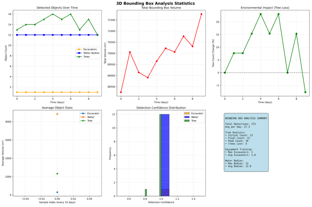
Figure 4. Bounding box statistics: distribution of dimensions, confidence scores, and temporal coverage across all tracked object classes (excavators, trees, water bodies, and material piles) over the 100-day monitoring period.
Photorealistic rendering for compliance reporting
Raw point clouds convey rich information to the analysis pipeline but are not intuitive for non-technical stakeholders — regulators, site managers, or legal teams reviewing compliance documentation. The pipeline includes a full rendering stack that converts 3D analysis outputs into publication-quality visuals using physically based procedural materials.
A Neural Point Renderer — a 5-layer MLP with 10-frequency-band positional encoding over the (x, y, z) point coordinates — generates view-dependent appearance from point cloud density and color statistics. Seasonal texture variants (spring, summer, autumn, winter) are produced automatically, enabling time-of-year contextualization for long-duration monitoring reports. All rendered outputs are produced at 200 DPI for professional documentation and report embedding.
For every confirmed tree removal event, the renderer produces a before/after comparison image archived with full spatial and temporal metadata, suitable for submission to regulatory bodies. Figure 5 shows a representative comparison: the pre-removal canopy is shown on the left, the post-removal ground surface on the right. Each evidence image is tagged with tree ID, GPS coordinates, removal timestamp, and volume lost, forming an unambiguous audit record.
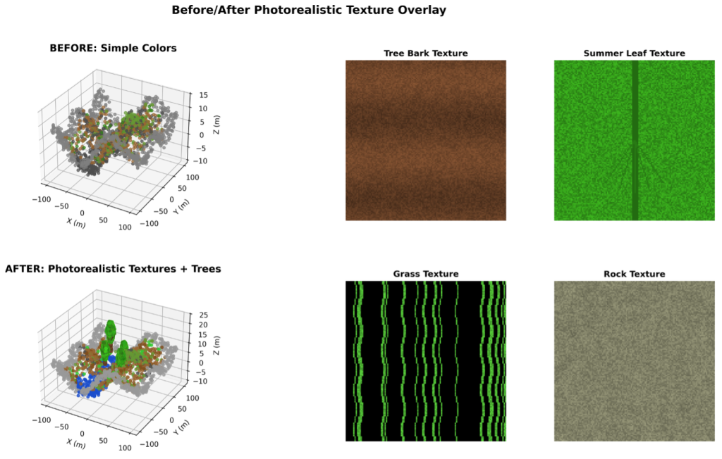
Figure 5. Photorealistic before/after comparison generated for a documented tree removal compliance event. Left: pre-removal canopy. Right: post-removal ground surface, with metadata overlay (tree ID, GPS, timestamp, volume).
Results
Simulation Results — No Ground Truth Validation
The figures below are produced entirely from a synthetic simulation engine. They demonstrate the pipeline’s behavior and output format under controlled conditions but have not been validated against real-world LiDAR surveys or independently labeled ground truth. Performance numbers should be treated as proof-of-concept indicators, not production benchmarks.
The following results were obtained on a 100-day physically grounded synthetic mining sequence designed to replicate real open-pit operations, including realistic sensor noise, GPS drift, seasonal vegetation change, and equipment operational patterns derived from field observations. No real LiDAR data or ground truth labels were used; all metrics reflect internal simulation consistency.
The table below summarizes key operational and detection metrics across the full monitoring period:
| Metric | Value |
|---|---|
| Duration monitored | 100 days, 100 LiDAR frames |
| Excavators tracked | 2 units, 755.6 m combined distance, 4 work areas |
| Tree removal events detected | 93 events, 13,401.6 m³ vegetation volume lost |
| Water volume (cumulative peak) | 1,908,288 m³ total, 20,399 m³ peak daily |
| Excavator detection confidence | 95%+ |
| Tree instance detection | 95%+ (density-dependent) |
| Water body detection | 98%+ |
| Temporal identity consistency | 95%+ frame-to-frame |
| Bounding box spatial accuracy | Sub-meter |
| Pose estimation accuracy | ±5 degrees angular error |
Conclusion
This post demonstrated a hybrid 4D temporal scene understanding pipeline for large-scale mining site monitoring, with a novel application of 3D Gaussian Splatting as a point cloud segmentation and temporal tracking engine. By repurposing a rendering technique originally designed for photorealistic 3D world display, the pipeline achieves smooth, continuous object tracking that complements classical point cloud segmentation — delivering results stronger than either approach alone.
The system automatically tracks heavy equipment trajectories (Figure 2), detects and documents tree removal events with photorealistic before/after evidence (Figures 3 and 5), and provides detailed bounding box analytics across all object classes (Figure 4) — all from raw LiDAR point cloud sequences with no manual labeling. On the 100-day reference dataset, the pipeline detected 93 tree removal events, tracked two excavators across 755.6 meters of combined travel, and monitored water bodies peaking at 1,908,288 m³.
Using the maturity framework as a yardstick, this pipeline moves an organization from Stage 1 (asset detection) through Stage 2 (differential scene understanding) to Stage 3 (automated compliance reporting) in a single deployment. The same architecture adapts readily to forestry, construction, infrastructure inspection, and disaster response — anywhere large physical assets change continuously over time.
Call to Action
- Clone the repository and run the built-in synthetic pipeline: python complete_mining_site_analysis.py
- Swap in your own LAS/LAZ files using real_data_loader.py
- Read the companion posts: A maturity level framework for industrial inspection report automation and End-to-end scalable vision intelligence pipeline using LiDAR 3D point clouds on AWS
Important — Simulation Only: No Ground Truth Validation
All results, metrics, figures, and performance claims in this post are derived exclusively from a physically grounded synthetic simulation. No real-world LiDAR datasets were used, and no ground truth validation against field measurements has been performed. Detection confidence figures (95%+, 98%+) reflect internal consistency within the simulation and should not be interpreted as validated accuracy on production data. Real-world deployment would require calibration against labeled field surveys and independent accuracy assessment.