AWS Big Data Blog
Get started with Amazon OpenSearch Service: T-shirt size your domain for log analytics
When you’re spinning up your Amazon OpenSearch Service domain, you need to figure out the storage, instance types, and instance count; decide the sharding strategies and whether to use a cluster manager; and enable zone awareness. Generally, we consider storage as a guideline for determining instance count, but not other parameters. In this post, we offer some recommendations based on T-shirt sizing for log analytics workloads.
Log analytics and streaming workload characteristics
When you use OpenSearch Service for your streaming workloads, you send data from one or more sources into OpenSearch Service. OpenSearch Service indexes your data in an index that you define.
Log data naturally follows a time series pattern, and therefore a time-based indexing strategy (daily or weekly indexes) is recommended. For efficient management of log data, you must implement time-based index patterns and set retention periods. You further define time slicing and a retention period for the data to manage its lifecycle in your domain.
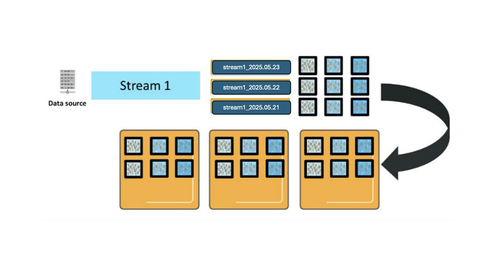
For illustration, consider that you have a data source producing a continuous stream of log data, and you’ve configured a daily rolling index and set a retention period of 3 days. As the logs arrive, OpenSearch Service creates an index per day with names like stream1_2025.05.21, stream1_2025.05.22, and so on. The prefix stream1_* is what we call an index pattern, a naming convention that helps group-related indexes.
The following diagram shows three primary shards for each daily index. These shards are deployed across three OpenSearch Service data instances, with one replica for each primary shard. (For simplicity, the diagram doesn’t show that primary and replica shards are always placed on different instances for fault tolerance.)
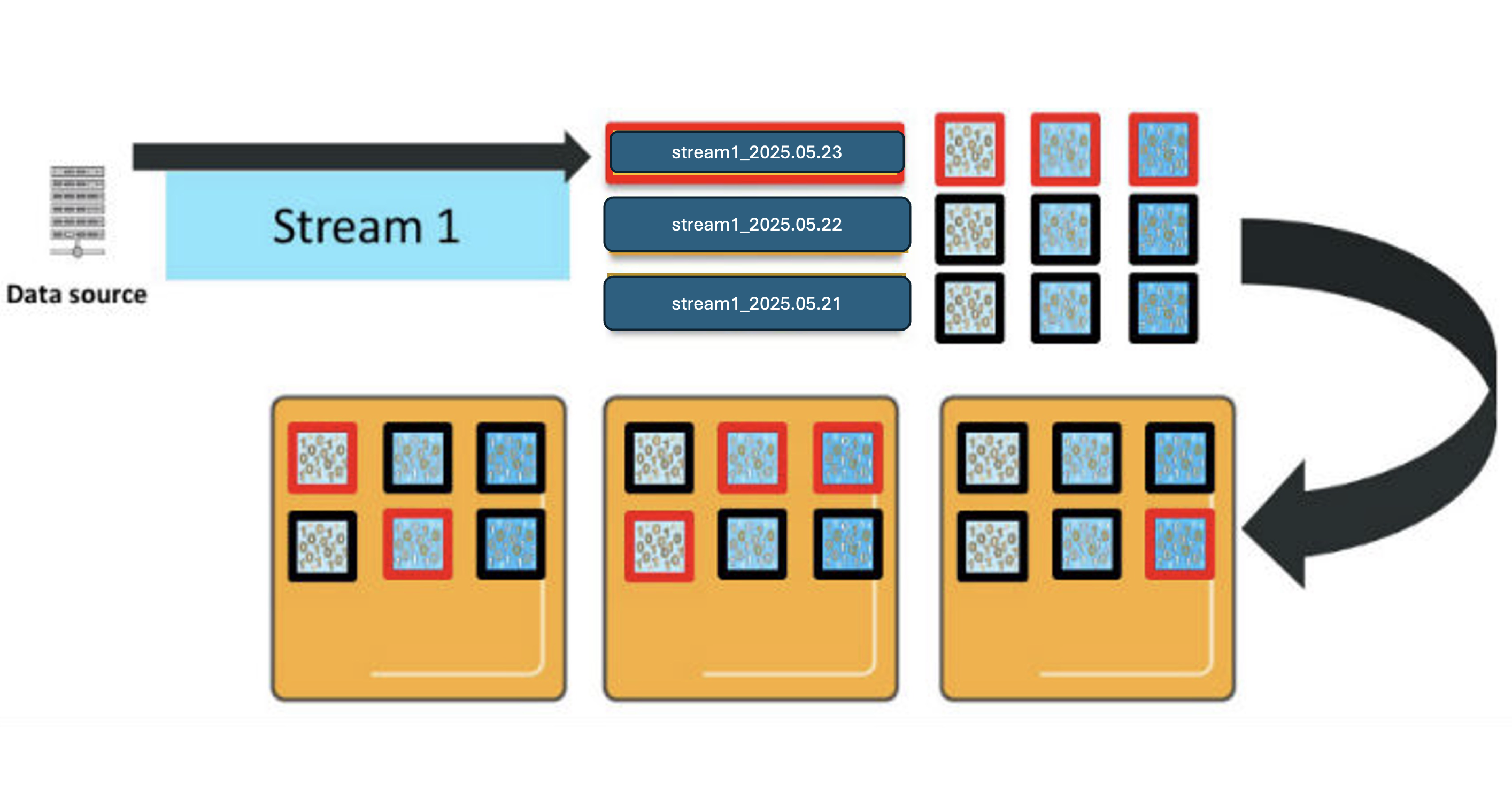
When OpenSearch Service processes new log entries, they are sent to all relevant primary shards and their replicas in the active index, which in this example is only today’s index due to the daily index configuration.
There are several important characteristics of how OpenSearch Service processes your new entries:
- Total shard count – Each index pattern will have a D * P * (1 + R) total shards, where D represents retention in days, P represents primary shards, and R is the number of replicas. These shards are distributed across your data nodes.
- Active index – Time slicing means that new log entries are only written to today’s index.
- Resource utilization – When sending a _bulk request with log entries, these are distributed across all shards in the active index. In our example with three primary shards and one replica per shard, that’s a total of six shards processing new data simultaneously, requiring 6 vCPUs to efficiently handle a single
_bulkrequest.
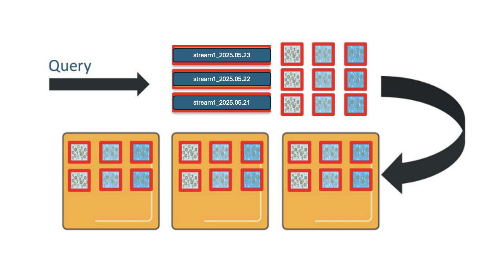
Similarly, OpenSearch Service distributes queries across the shards for the indexes involved. If you query this index pattern across all 3 days, you will engage 9 shards, and need 9 vCPUs to process the request.
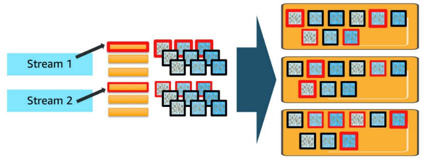
This will get even more complicated when you add in more data streams and index patterns. For each additional data stream or index pattern, you deploy shards for each of the daily indexes and use vCPUs to process requests in proportion to the shards deployed, as shown in the preceding diagram. When you make concurrent requests to more than one index, each shard for all the indexes involved must process those requests.
Cluster capacity
As the number of index patterns and concurrent requests increases, you can quickly overwhelm the cluster’s resources. OpenSearch Service includes internal queues that buffer requests and mitigate this concurrency demand. You can monitor these queues using the _cat/thread_pool API, which shows queue depths and helps you understand when your cluster is approaching capacity limits.
Another complicating dimension is that the time to process your updates and queries depends on the contents of the updates and queries. As requests come in, the queues are filling at the rate you are sending them. They are draining at a rate that is governed by the available vCPUs, the time they take on each request, and the processing time for that request. You can interleave more requests if those requests clear in a millisecond than if they clear in a second. You can use the _nodes/stats OpenSearch API to monitor average load on your CPUs. For more information about the query phases, refer to A query, or There and Back Again on the OpenSearch blog.
If you see the queue depths increasing, you are moving into a “warning” area, where the cluster is handling load. But if you continue, you can start to exceed the available queues and must scale to add more CPUs. If you start to see load increasing, which is correlated with queue depth increasing, you are also in a “warning” area and should consider scaling.
Recommendations
For sizing a domain, consider the following steps:
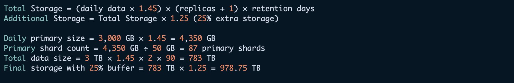
- Determine the storage required – Total storage = (daily source data in bytes × 1.45) × (number_of_replicas + 1) × number of days retained. This accounts for the additional 45% overhead on daily source data, broken down as follows:
- 10% for larger index size than source data.
- 5% for operating system overhead (reserved by Linux for system recovery and disk defragmentation protection).
- 20% for OpenSearch reserved space per instance (segment merges, logs, and internal operations).
- 10% for additional storage buffer (minimizes impact of node failure and Availability Zone outages).
- Define the shard count – Approximate number of primary shards = storage size required per index / desired shard size. Round up to the nearest multiple of your data node count to maintain even distribution. For more detailed guidance on shard sizing and distribution strategies, refer to “Amazon OpenSearch Service 101: How many shards do I need” For log analytics workloads, consider the following:
- Recommended shard size: 30–50 GB
- Optimal target: 50 GB per shard
- Calculate CPU requirements – Recommended ratio is 1.25 vCPU:1 Shard for lower data volumes. Higher ratios are recommended for larger volumes. Target utilization is 60% average, 80% maximum.
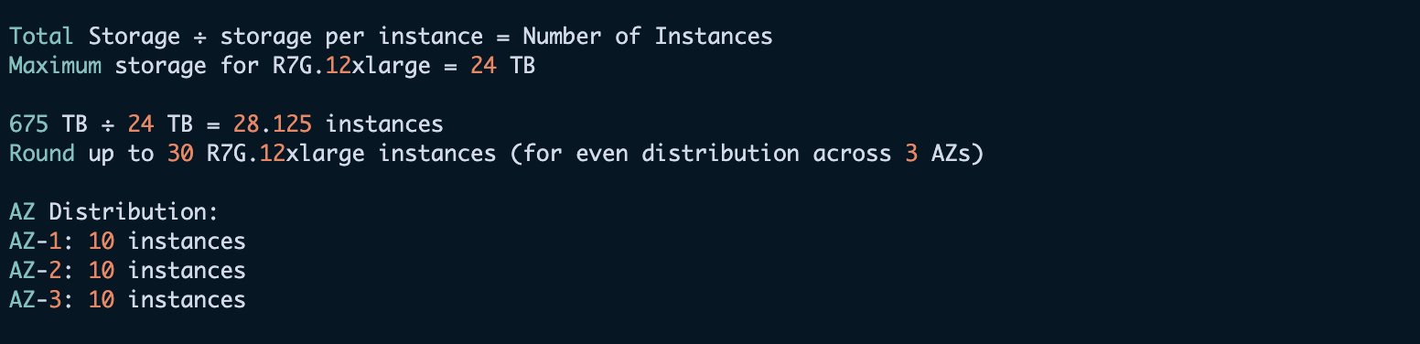
- Choose the right instance type – Consider the following based on your nodes:
- Cluster manager nodes: M family AWS Graviton instances (all workload sizes)
- Data nodes (small to large workloads): M or R family AWS Graviton instances with Amazon Elastic Block Store (Amazon EBS)
- Data nodes (very large workloads): I family instances with NVMe SSDs
Let’s look at an example for domain sizing. The initial requirements are as follows:
- Daily log volume: 3 TB
- Retention period: 3 months (90 days)
- Replica count: 1
We make the following instance calculation.
The following table recommends instances, amount of source data, storage needed for 7 days of retention, and active shards based on the preceding guidelines.
| T-Shirt Size | Data (Per Day) | Storage Needed (with 7 days Retention) | Active Shards | Data Nodes | Primary Nodes |
| XSmall | 10 GB | 175 GB | 2 @ 50 GB | 3 * r7g.large. search | 3 * m7g.large. search |
| Small | 100 GB | 1.75 TB | 6 @ 50 GB | 3 * r7g.xlarge. search | 3 * m7g.large. search |
| Medium | 500 GB | 8.75 TB | 30 @ 50 GB | 6 * r7g.2xlarge.search | 3 * m7g.large. search |
| Large | 1 TB | 17.5 TB | 60 @ 50 GB | 6 * r7g.4xlarge.search | 3 * m7g.large. search |
| XLarge | 10 TB | 175 TB | 600 @ 50 GB | 30 * i4g.8xlarge | 3 * m7g.2xlarge.search |
| XXL | 80 TB | 1.4 PB | 2400 @ 50 GB | 87 * I4g.16xlarge | 3 * m7g.4xlarge.search |
As with all sizing recommendations, these guidelines represent a starting point and are based on assumptions. Your workload will differ, and so your actual needs will differ from these recommendations. Make sure to deploy, monitor, and adjust your configuration as needed.
For T-shirt sizing the workloads, an extra-small use case encompasses 10 GB or less of data per day from a single data stream to a single index pattern. A small use case falls between 10–100 GB per day of data, a medium use case between 100–500 GB of data, and so on. Default instance count per domain is 80 for most of the instance family. Refer to the “Amazon OpenSearch Service quotas “ for details.
Additionally, consider the following best practices:
- Choose the right storage tier [Ultra Warm, Hot storage] for your needs in OpenSearch Service. Refer to the Choose the right storage tier for your needs in Amazon OpenSearch Service for details.
- Use the OpenSearch Optimized (OR) family for large-scale workloads that require low latency with index-heavy operations. Refer to OpenSearch optimized instance (OR1) is game changing for indexing performance and cost for details.
- Isolate the ingestion using an OpenSearch Ingestion pipeline for smaller to large workloads and reduce the operational overhead of managing the ingestion pipelines.
- Use reserved instances for long-term cost savings.
- Consider using Availability Zone awareness for high availability.
Conclusion
This post provided comprehensive guidelines for sizing your OpenSearch Service domain for log analytic workloads, covering several critical aspects. These recommendations serve as a solid starting point, but each workload has unique characteristics. For optimal performance, consider implementing additional optimizations like data tiering and storage tiers. Evaluate cost-saving options such as reserved instances, and scale your deployment based on actual performance metrics and queue depths.By following these guidelines and actively monitoring your deployment, you can build a well-performing OpenSearch Service domain that meets your log analytics needs while maintaining efficiency and cost-effectiveness.