Containers
Data-driven Amazon EKS cost optimization: A practical guide to workload analysis
This post introduces some of the key considerations for optimizing Amazon Elastic Kubernetes Service (Amazon EKS) costs in production environments. Through detailed workload analysis and comprehensive monitoring, we demonstrate a proven best practice to maximize cost savings while maintaining performance and resilience supported by real-world examples and practical implementation guidelines.
Common pattern of resource waste
In pursuing optimal performance and resilience, organizations often struggle to balance cost efficiency, as shown in the following figure.
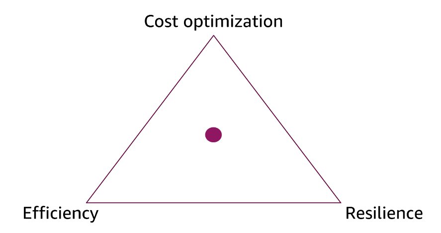
Figure 1: Strategic balance triangle showing trade-offs
Through collaboration with application owners and developers, a clear pattern emerges: the primary driver of cloud cost waste is overprovisioned resources, justified by performance and resilience considerations that may no longer reflect actual needs. In this post we discuss three critical areas of waste:
Greedy workload: oversized pod resources for performance
Pet workload: excessive replica counts for resilience
Isolated workload: fragmented node pools with stranded capacity for performance
Each decision, made with good intentions, accumulates into unnecessary spending over time. The challenge is finding the optimal balance through data-driven rightsizing and architectural optimization.
The greedy workload caused oversized pod resources
Problem:
We can call them greedy workloads if a Pod’s requests are higher than what the application actually tries to use.
The application tries to actually use ~0.2vCPU (200 m) and ~1 Gi of memory.
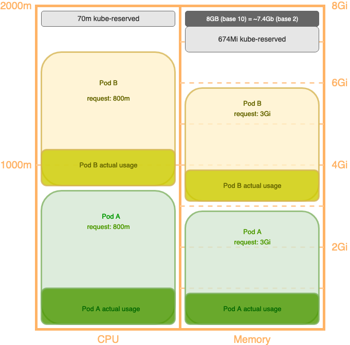
Figure 2: Request and actual usage
Impact:
We can see that in total we’re actually only using ~400 m/1930 m (~21%) vCPU, and ~2 Gi/6.8 Gi (~29%) memory, as shown in the preceding figure.
Despite having plenty of actual resources for more copies of this Pod, Kubernetes doesn’t place any more replicas on this node because the allocatable resources have been almost completely allocated.
Resolution:
We adjust the requests to be 200 m CPU and 1 Gi of memory to match the application’s workload.
When placing the updated Pods, we can now place 6 Pods per node! In total we’re now actually using 1200 m/1930 m (~62%) vCPU, and ~6 Gi/6.8 Gi (~88%) memory per node.
When compared to the previous one, this node can now take 3 times the Pods as it did before. We should only need one third of the Amazon Elastic Compute Cloud (Amazon EC2) instances to run this same workload, as shown in the following figure.
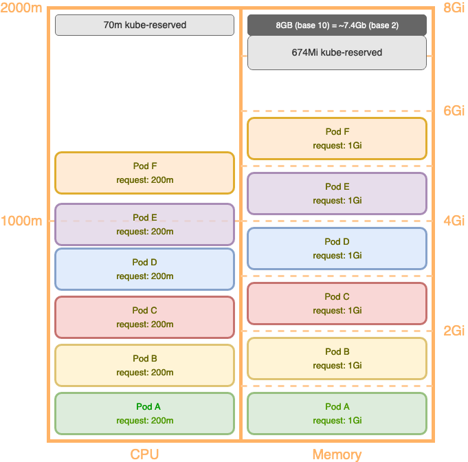
Figure 3: Configure appropriate resource requests to improve utilization
Recommendations:
- Pod Requests should be configured to accurately reflect the resource usage of the application under ideal load.
- Consider removing CPU limits from pods or setting them with caution because it impacts application performance when resources are available. Refer to this post for additional details: Using Prometheus to Avoid Disasters with Kubernetes CPU Limits
- Set memory
requests= memorylimitsto a avoid resource contention on bursty workloads.
Tools to help with this:
- Kubecost: Kubecost launched to provide customers with visibility into spend and resource efficiency in Kubernetes environments. Kubecost has a premium tier, but Amazon EKS customers can install a tailored package. Refer to this post for additional details. AWS and Kubecost Collaborate to Deliver Kubecost 2.0 for Amazon EKS Users
- Goldilocks: We use the kubernetes vertical-Pod-autoscaler in recommendation mode and observe a suggestion for resource requests on each of our apps. This tool creates a VPA for each workload in a namespace and queries them for information.
- Vertical Pod Autoscaler: can recommend or automatically adjust Pod requests based on their observed usage.
- Prometheus metrics:
- KubeCost leans on
kube-state-metrics. If you already have the prometheus metrics in your cluster, then you could adapt their queries. - Grafana Dashboard based on similar queries.
- KubeCost leans on
The pet workload causes excessive replica counts
Problem:
The pet workload is configured with some specific settings because of resilience considerations. The following are some examples:
- Overly strict pod disruption budgets
- Overly strict topology spread constraints
- Stateful apps without restart support
- Critical, stateful workloads ran for extended periods with “do not disrupt” labels to prevent interruption.
Impact:
These long-lived pet workloads effectively block node consolidation, resulting in underused but non-disruptible nodes. Furthermore, high-frequency short-running jobs continue to reset the “last pod event time” on nodes, preventing Karpenter from consolidating them even when they are mostly idle.
Overly strict topology spread constraints:
You can use topology spread constraints to control how pods are spread across your cluster among failure-domains such as AWS Regions, zones, nodes, and other user-defined topology domains.
Scenario 1: (maxSkew = 1): Needs 7 total pods distributed as [2, 2, 1, 2] across four AWS Availability Zones (AZs). The strict maxSkew=1 constraint means that no zone can have more than 1 pod difference from any other zone. This forces the scheduler to maintain near-perfect balance. The actual skew achieved is 1 (max 2 pods, min 1 pod).
Scenario 2: (maxSkew = 3): Needs only 4 total pods distributed as [1, 3, 0, 0], using just two AZs. The relaxed maxSkew=3 constraint allows up to 3 pods difference between zones, enabling maximum flexibility in placement. The actual skew is 3 (max 3 pods, min 0 pods).
Recommendation:
You can change the maxSkew from 1 to 3 to reduce the replica count from 7 to 4 pods—a 43% reduction (3 fewer pods). This translates directly to lower compute costs while still maintaining reasonable availability, because pods remain distributed across multiple zones. The trade-off is significantly relaxed zone balancing, but for cost-sensitive workloads this constraint still provides adequate fault tolerance by keeping pods in at least two different AZs, all while achieving substantial cost savings.
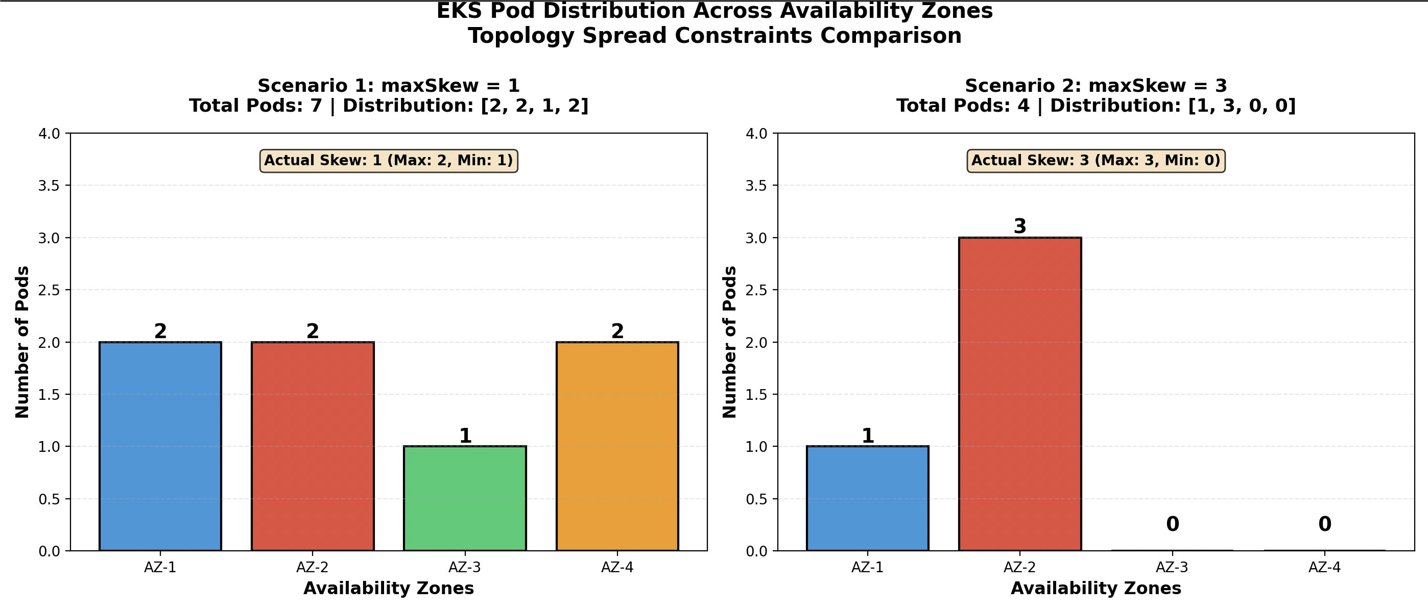
Figure 4: Distribute pods across availability zones using Topology Spread Constraints
Overly strict Pod Distribution Budget (PDB):
When customers configure overly restrictive PDBs with a low maxUnavailable count, they prevent potential voluntary pod evictions, including those needed for:
- Karpenter node consolidation
- Routine node maintenance and patching
- Cluster optimization operations
This blocks cost-saving opportunities and can also degrade overall cluster health by preventing necessary infrastructure updates.
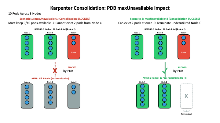
Figure 5: Overly strict PDB settings can block Karpenter node consolidation
Recommendations:
- Optimize Topology Spread Constraints based on actual resilience requirements rather than theoretical maximums.
- Provide sensible default PDB configurations for applications that lack explicit policies. Make sure that defaults protect against disruptions without being overly restrictive.
- Regularly audit and review workloads with this annotation to prevent overuse that impedes cost optimization. Restrict use of karpenter.sh/do-not-disrupt annotation to justified cases only.
- If restrictive PDBs have to be in place for certain applications, then evaluate the terminationGracePeriod set up to forcibly clean up the node.
The isolated workloads configured with fragmented node pools
When you first installed Karpenter, you set up a default NodePool. The NodePool sets constraints on the nodes that can be created by Karpenter and the pods that can run on those nodes.
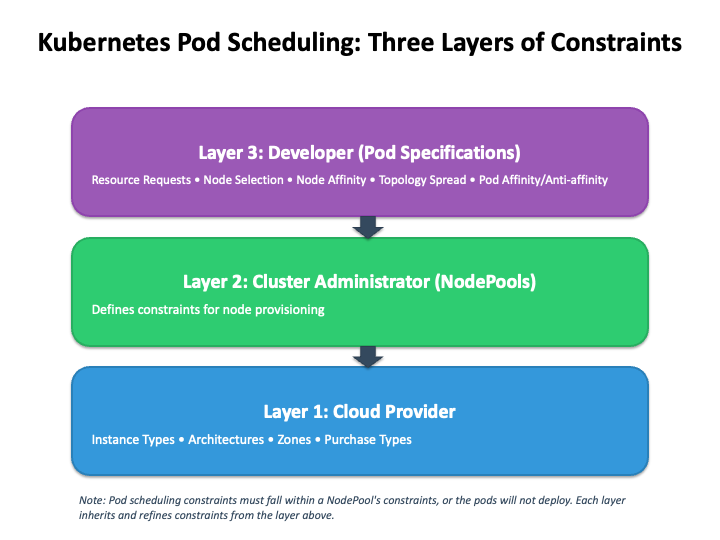
Figure 6: Three layer of constraints for Kubernetes pod scheduling
This preceding figure shows the three-layer hierarchy of constraints in Kubernetes pod scheduling. At the foundation (bottom), the Cloud Provider layer establishes baseline constraints, including available instance types, architectures, zones, and purchase options. The middle layer shows how Cluster Administrators use NodePools to add more constraints for node provisioning and pod placement, which must operate within the Cloud Provider’s limitations. At the top, Developers specify pod-level constraints such as resource requests, node selection, affinity rules, and topology spread requirements. All of these must comply with both the NodePool and Cloud Provider constraints beneath them. The downward-pointing arrows emphasize that each layer inherits and refines constraints from the layers beneath it, creating a cascading constraint system where pods can only be scheduled if their specifications align with all three layers.
The following strategies are for defining nodepools.
Single NodePool strategy: Uses one NodePool to manage compute resources for multiple teams and workloads. This is useful when you want a direct setup, such as a single NodePool that handles both AWS Graviton and x86 instances while allowing pods to specify their processor requirements.
Multiple NodePool strategy: Creates separate NodePools to isolate compute resources for different purposes. Example use cases include isolating expensive hardware, maintaining security boundaries between workloads, separating teams, using different Amazon Machine Images (AMIs), using different NodePool disruption budgets, or preventing noisy neighbor issues through tenant isolation.
Weighted NodePool strategy: Defines a priority order across multiple NodePools so that the scheduler attempts to place pods in preferred NodePools first before falling back to others. This is particularly useful for cost optimization scenarios such as prioritizing Reserved Instances and Savings Plans over on-demand instances, setting default cluster-wide configurations, or maintaining specific ratios between Spot/On-Demand instances or x86/Graviton processors.
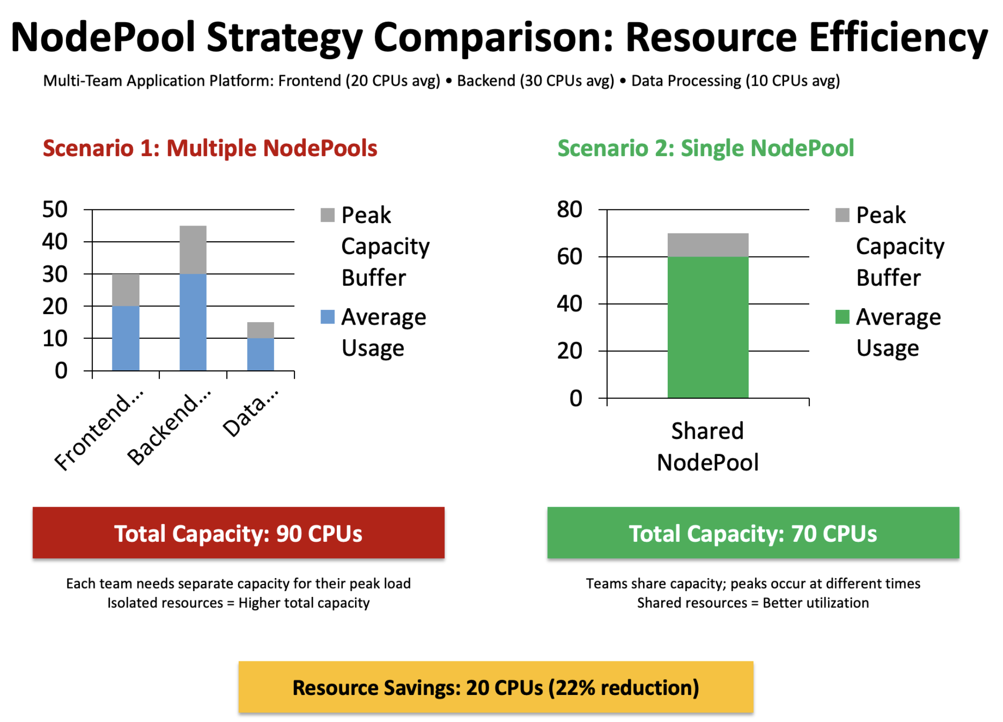
Figure 7: Optimize NodePool settings to improve resource efficiency
The preceding graph compares resource efficiency between two NodePool strategies for a multi-team platform.
On the left, Scenario 1 (Multiple NodePools) shows three separate columns representing isolated NodePools for Frontend, Backend, and Data Processing teams. Each one must provision enough capacity to handle its own peak load, resulting in a total capacity requirement of 90 CPUs.
On the right, Scenario 2 (Single NodePool) displays one unified column where all teams share a common pool that only needs 70 CPUs total. This achieves the same workload coverage with less overall capacity.
Why the savings occur:
- Peak load smoothing: Teams peak at different times, so the single pool handles the aggregate peak rather than sum of individual peaks.
- No capacity fragmentation: Unused capacity in one team’s pool can be used by another team.
- Reduced buffer requirements: Instead of each pool maintaining its own safety buffer, one shared buffer is sufficient.
Recommendations:
- The choice of strategy depends on your organization’s needs for workload isolation, cost optimization, and operational complexity.
- When possible, define constraints at Layer 3 (pod specification level) rather than creating more NodePools at Layer 2, because this maintains flexibility and reduces infrastructure complexity.
- We recommend creating NodePools that are mutually exclusive. Therefore, no Pod should match multiple NodePools. If multiple NodePools are matched, then Karpenter uses the NodePool with the highest weight.
Conclusion
Optimizing Amazon EKS costs isn’t about cutting corners—it’s about eliminating waste while preserving performance and reliability. You can use data-driven rightsizing to identify and eliminate overprovisioned resources that drain budgets without adding value. When you combine this with architectural optimization strategies such as thoughtful NodePool design and strategic constraint placement, you can achieve substantial cost reductions while maintaining operational excellence.
About the authors
 Frank Fan is a Sr. Container Solutions Architect at AWS Australia. As a passionate advocate for application modernization, Frank specializes in containerization and overseeing large-scale migration and modernization initiatives. Frank is a frequent speaker at prominent tech events including AWS reInvent, AWS Summit and Kubernetes Community Day. You can get in touch with Frank via his LinkedIn page, and his presentations are available at his YouTube channel
 Alan Halcyon is a Senior Specialist Technical Account Manager at AWS in the Containers domain. He helps AWS customers optimize and troubleshoot large scale Kubernetes workloads, and loves the weird or difficult problems.
 Angela Wang is a Technical Account Manager based in Australia with over 10 years of IT experience, specializing in cloud-native technologies and Kubernetes. She works closely with customers to troubleshoot complex issues, optimize platform performance, and implement best practices for cost optimized, reliable and scalable cloud-native environments. Her hands-on expertise and strategic guidance make her a trusted partner in navigating modern infrastructure challenges.