AWS Database Blog
Amazon Aurora DSQL observability concepts and usage with Amazon CloudWatch
Amazon Aurora DSQL now offers enhanced observability through Amazon CloudWatch Database Insights, giving you time-based performance diagnostics that connect directly to what you experience and what you pay.
Observability in Amazon Aurora DSQL aims to provide clearly actionable insights into the operation of a DSQL cluster. This post covers the observability model, its connection to performance and cost, and how to use CloudWatch Database Insights, PromQL, and the DSQL system diagnostics AI skill in practice.
Why time-based observability?
Aurora DSQL uses an on-demand pricing model based on DPU (Distributed Processing Units), which reflects the time and resources dedicated to processing your requests. As a result, with DSQL you only accrue DPU when your database is doing work on your behalf. This billing model makes it critical to understand where your sessions spend their time, which is exactly what the DSQL observability model shows you.
DSQL observability is focused on giving you a clear, direct signal that answers the question every developer cares about: Where is my time being spent? It is largely built around the concept of time, providing a direct link between what you observe and what you experience. Time is the unit that matters most for performance. It also correlates directly with the DSQL on-demand pricing model: You pay only for what you use. This is entirely deliberate, because this correlation means you can manage your costs in lockstep with observable performance. Faster queries consume fewer DPU.
DSQL builds on a proven approach. Time-based observability has demonstrated success across many databases over several years, including commercial databases, PostgreSQL, and MySQL. DSQL brings this same proven model to a distributed SQL environment, natively, without also creating potential confusion by way of hundreds of counters.
An introduction to DASH
DSQL Active Session History (DASH) powers the observability metrics by monitoring the activity of sessions in the cluster. DASH samples every active session in the cluster every second and publishes 1-min aggregated data points as CloudWatch OTel metrics. A session is considered active if any of the following are true:
- The session is actively consuming CPU.
- The session is blocked on a wait event (such as storage waits or commit waits).
- The session is in a transaction but waiting for a request from the application.
These conditions all contribute to transaction latency and DPU, the DSQL billing unit that largely reflects the amount of time spent processing queries. Because DPU is proportional to active session time, decreasing the time your queries spend waiting (or processing inefficiently) translates directly into cost savings.
Each sample taken includes additional context, most notably the first 256 characters of the SQL text that was executing at the time of that sample. This means we know what was running and what it was waiting on at the time the sample was taken.
DASH samples once per second, which might seem coarse at first glance. In practice, this frequency answers the fundamental question: Where is the time going in my cluster? DASH provides a probabilistic view that minimizes diagnosis overhead and reliably surfaces the root cause in most performance diagnostics scenarios. The PromQL examples shown later in this post demonstrate this in practice.
All Aurora DSQL clusters include DASH enabled by default at no additional cost, providing observability data from the moment you create your cluster.
CloudWatch Database Insights
Amazon CloudWatch Database Insights provides an intuitive way to consume DASH data. It answers two key questions: where are my sessions spending most of their time, and which SQL statements are the most active?
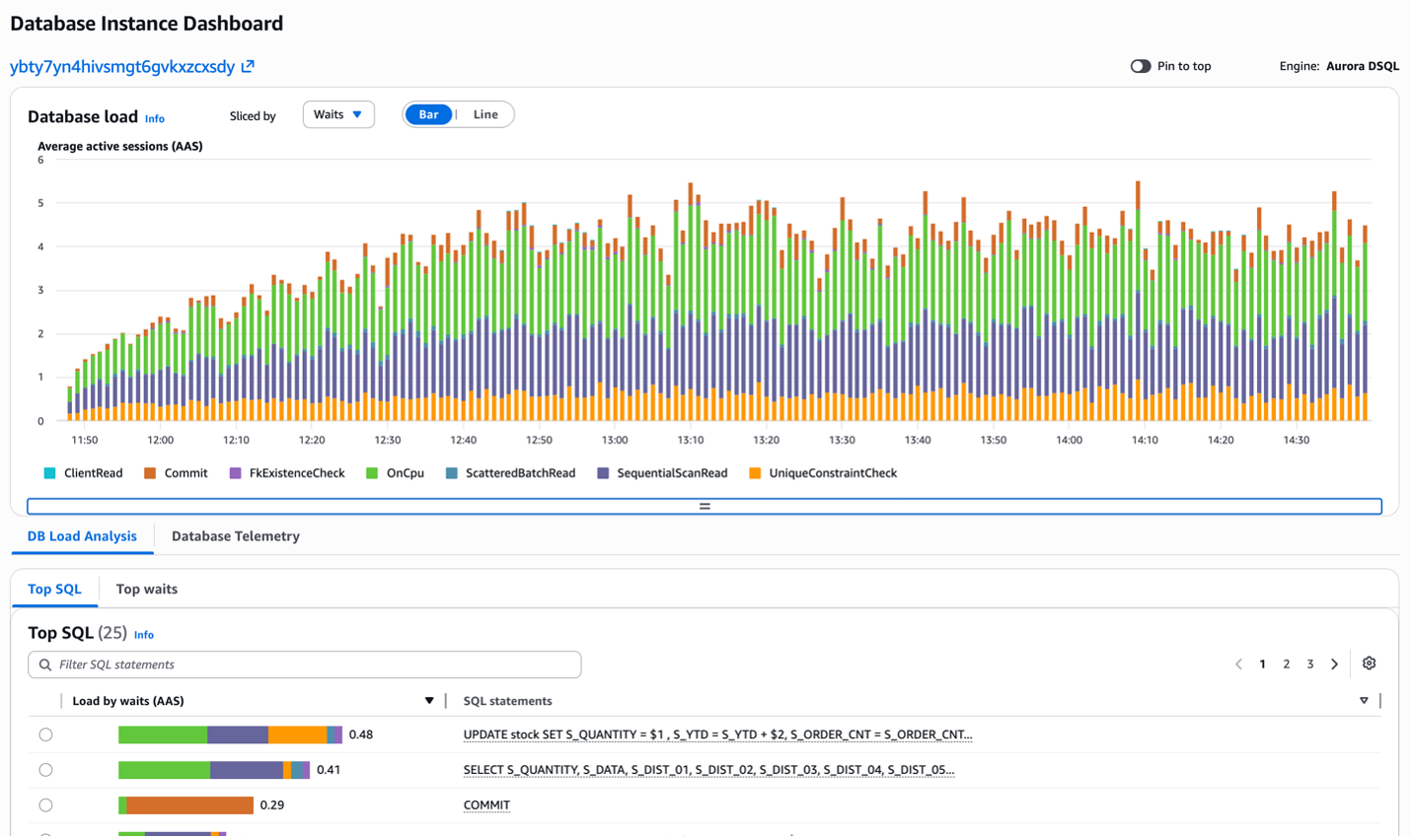
Figure 1: CloudWatch Database Insights showing database load by wait event and the most active SQL statements
AWS provides CloudWatch Database Insights Standard Mode with 1-minute metrics for Aurora DSQL at no additional charge, and enables it by default on all clusters. DSQL retains DASH data for 15 months. This gives you a deep historical window for trend analysis, capacity planning, and investigating intermittent issues that might only surface over longer time periods.
CloudWatch Database Insights shows the same familiar view that Amazon Relational Database Service (Amazon RDS) and Amazon Aurora (non-DSQL) databases show. The upper pane shows the DBLoad timeline using Average Active Sessions (AAS) for wait events that were sampled during that period.
A notable difference from RDS and Aurora (non-DSQL) databases is the absence of a Max vCPU line. Because DSQL scales elastically, there is no fixed capacity ceiling, so you determine system health differently, as discussed later in this post.
The lower pane shows the most active SQL during that period, defined by the number of Average Active Sessions executing that SQL statement at the time of the sample. Unlike RDS and Aurora, the DSQL view does not currently include drilldown to cumulative SQL statistics or execution plan information.
Wait events
DSQL wait events are few compared to, for example, community PostgreSQL. Although the list of wait events might increase over time to achieve better granularity, it is highly unlikely to ever get close to the 273 currently defined in PostgreSQL 18, for example. This is because the DSQL query processor (QP) doesn’t need to manage latches (LWLock), data locks, or IPC, which make up the majority of the defined wait events in community PostgreSQL. The following table describes the current list of DSQL wait events:
| Wait name | Description |
OnCpu |
The session is not waiting for external input and is actively executing on CPU. This includes parsing, planning, evaluating expressions, or processing results. |
ClientRead |
The session is idle within an open transaction, waiting for the application to send the next SQL statement or a commit/rollback command. Frequent or long ClientRead waits often indicate excessive application round-trips or transactions that are held open longer than necessary. |
ClientWrite |
Results are being sent from the database to the application over the network. High ClientWrite can indicate large result sets or network latency between the application and the database. |
Commit |
The session has initiated a commit and is waiting for acknowledgement from the commit service. The response is either a success or an abort (serialization error). Both outcomes are preceded by a Commit wait. |
FkExistenceCheck |
The session is validating that a referenced foreign key row exists, which requires reads to confirm the relationship. |
PgSleep |
The session is sleeping because the application explicitly called pg_sleep(). This is an application-initiated wait, not a database-imposed one. |
ScatteredBatchRead |
The session is performing batched reads from storage, retrieving multiple non-contiguous keys in a single call to storage. |
SequentialScanRead |
The session is reading a contiguous range of keys from storage. This is not necessarily a full table scan. It might cover a relatively small range of contiguous keys. |
SingleRead |
The session is reading a single tuple (point lookup) from storage. This event is largely replaced by ScatteredBatchRead with a batch size of 1 and is uncommon in current DSQL versions. |
StartTransaction |
The session is preparing for the distributed transaction to begin. |
UniqueConstraintCheck |
The session is validating unique key constraints, which requires storage reads to check for duplicates. This applies to both unique constraints on non-primary-key columns and primary key constraints during the insertion of new rows. |
Table 1: DSQL wait events
SQL statements
DSQL references SQL statements by Query ID, which is a base32 representation of the unique query ID generated by the QP based on the SQL text. DSQL assigns a Query ID to all SQL in the DASH data. Requests report their SQL text in a normalized form that replaces literal values with $-prefixed numeric identifiers.
Direct query with PromQL
PromQL is an alternative to using Database Insights to query the underlying DASH data directly. DSQL exposes DASH data as CloudWatch OTel metrics, which you can query using PromQL in Amazon CloudWatch Query Studio. This offers the same information as Database Insights, along with additional dimensions for custom analysis.
The following PromQL examples cover three common use cases. First, identifying which wait events accrue the most time. Second, finding the queries that spend the most time waiting. Third, pinpointing queries that wait longest on storage. Make sure to replace my_cluster_id with your real cluster ID before trying these queries in Query Studio.
Database load by Average Active Sessions
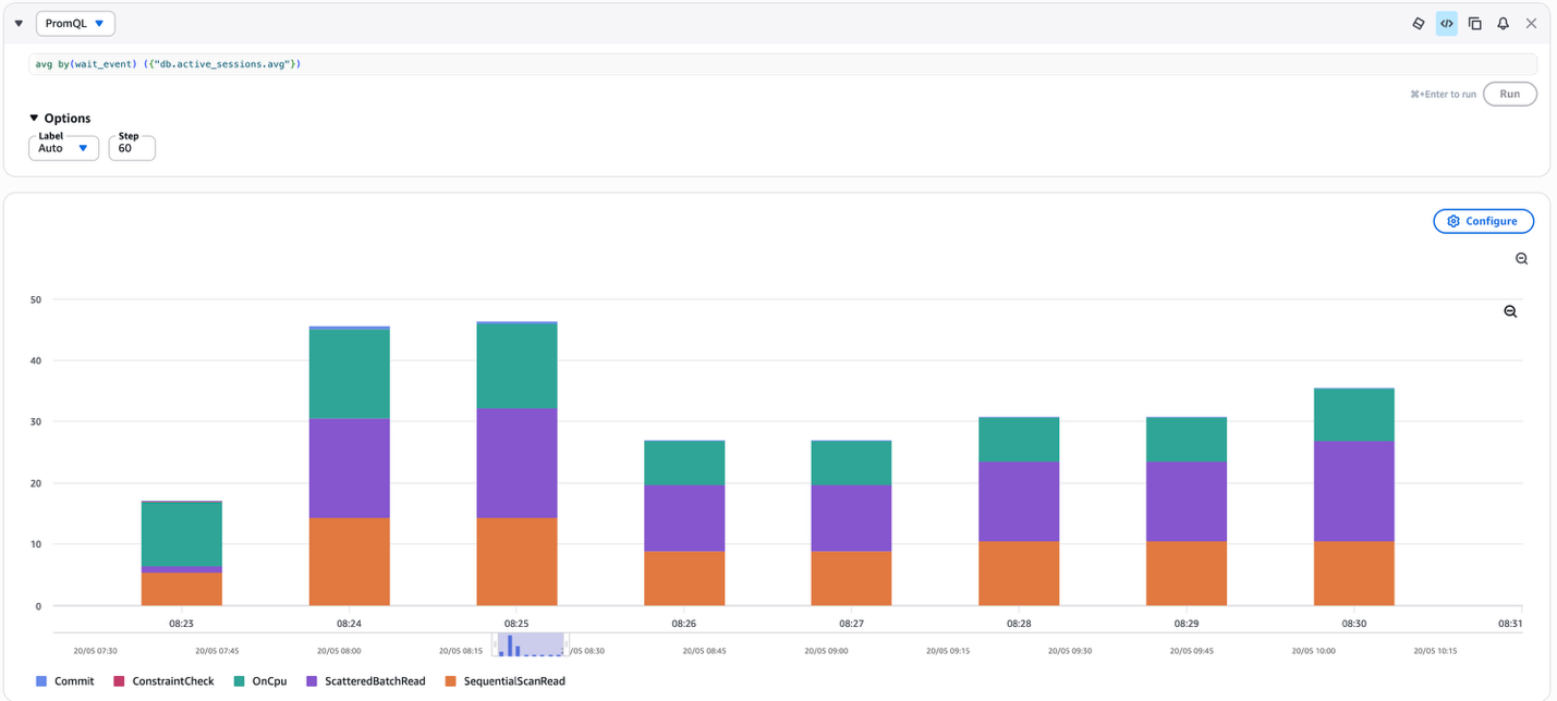
Figure 2: Database load by average active sessions, grouped by wait event
Top 5 queries by Average Active Sessions
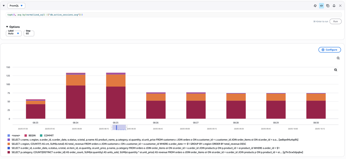
Figure 3: Top five queries by average active sessions
Top 5 queries by Average Active Sessions and wait event
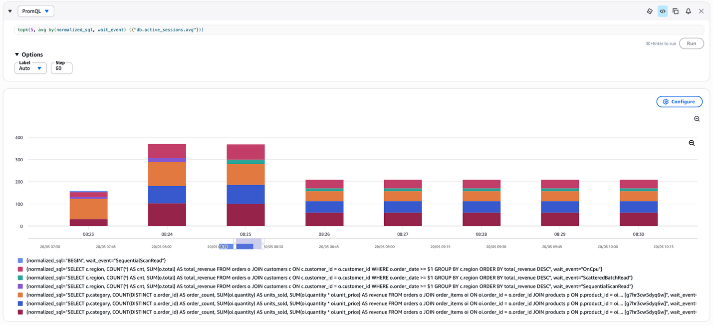
Figure 4: Top five queries by average active sessions and wait event
Top 5 queries by Average Active Sessions and storage waits
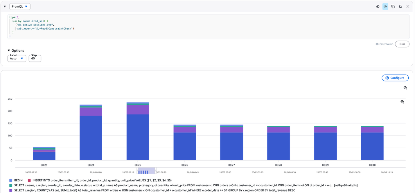
Figure 5: Top five queries by average active sessions and storage waits
Application health
In other AWS relational database services, having as many sessions on CPU as there are vCPUs in the instance is a sign of poor health. You observe poor latency when the demand from the application exceeds the available compute. As we described earlier, DSQL doesn’t have the concept of Max vCPU, because clusters scale elastically to match the demand, and so we need an alternative method for determining the health of the application.
Let’s start with what a healthy system looks like in terms of AAS: There is no single answer for this. It is specific to each application, and the load of that application. One application might behave normally when five sessions are concurrently active, waiting on storage reads, and behave poorly when there are 10 sessions waiting on storage reads. Another application might behave perfectly when there are 500 sessions waiting on storage reads. The important concept is that different applications have a distinct AAS profile for normal operation. Specific numbers of waiters do not, on their own, indicate poor health.
The elastic scaling nature of DSQL also means that 100 waiters one day and 1,000 the next does not necessarily signal poor health. It might simply mean the system is processing 10x more transactions. So how do we determine health?
The answer is that we must compare the proportions of wait events over time, rather than absolute numbers. For example, let’s assume a healthy application shows a wait profile like shown in the following table:
| Wait event | Waiter count |
SequentialScanRead |
40 |
Commit |
10 |
OnCpu |
50 |
Table 2: Normal wait event proportions
A busy day might bump those counts to 80, 20, 100 respectively. The relative proportions remain the same, indicating the system is twice as busy but still healthy. DSQL scales automatically to accommodate the additional load. However, if there is a day where the wait profile looks like the following table, we know that something has gone awry:
| Wait event | Waiter count |
SequentialScanRead |
90 |
Commit |
3 |
OnCpu |
7 |
Table 3: Abnormal wait event proportions
In this case, it is likely that an application change, or a SQL plan change, has caused the sessions to spend more of their time scanning data than processing and committing the changes. This is an unhealthy system, because the proportions of wait events have shifted dramatically away from the expected distribution.
This might seem complex. In reality, Database Insights makes this fast to process visually. Consistent color assignments help you quickly learn what normal operation looks like. Of course, visual checks are insufficient to properly manage a production system, and we recommend that you configure automated alarms. You can configure these alarms in CloudWatch as high/low band thresholds of AAS per wait event. For more elaborate analysis, run trend queries on the raw data to examine wait distribution over time.
DSQL system diagnostics AI skill
The databases-on-aws plugin, part of Agent Plugins for AWS, makes DSQL system diagnostics health checks easier. After it’s configured, you can request performance checks for your DSQL cluster across different timeframes. This triggers a workflow that uses the CloudWatch MCP server to analyze the DASH data over a selection of timeframes. Once installed in your agent, you can issue prompts such as:
“Check the performance of my DSQL cluster in us-east-1 and write me a markdown report”
The skill then compares against historical baselines. By default, these are the last hour, same hour yesterday, and same hour last week, but you can change them with prompts such as:
“Check performance for the last 4 hours and compare against last Monday”
An example of a Markdown report is as follows:
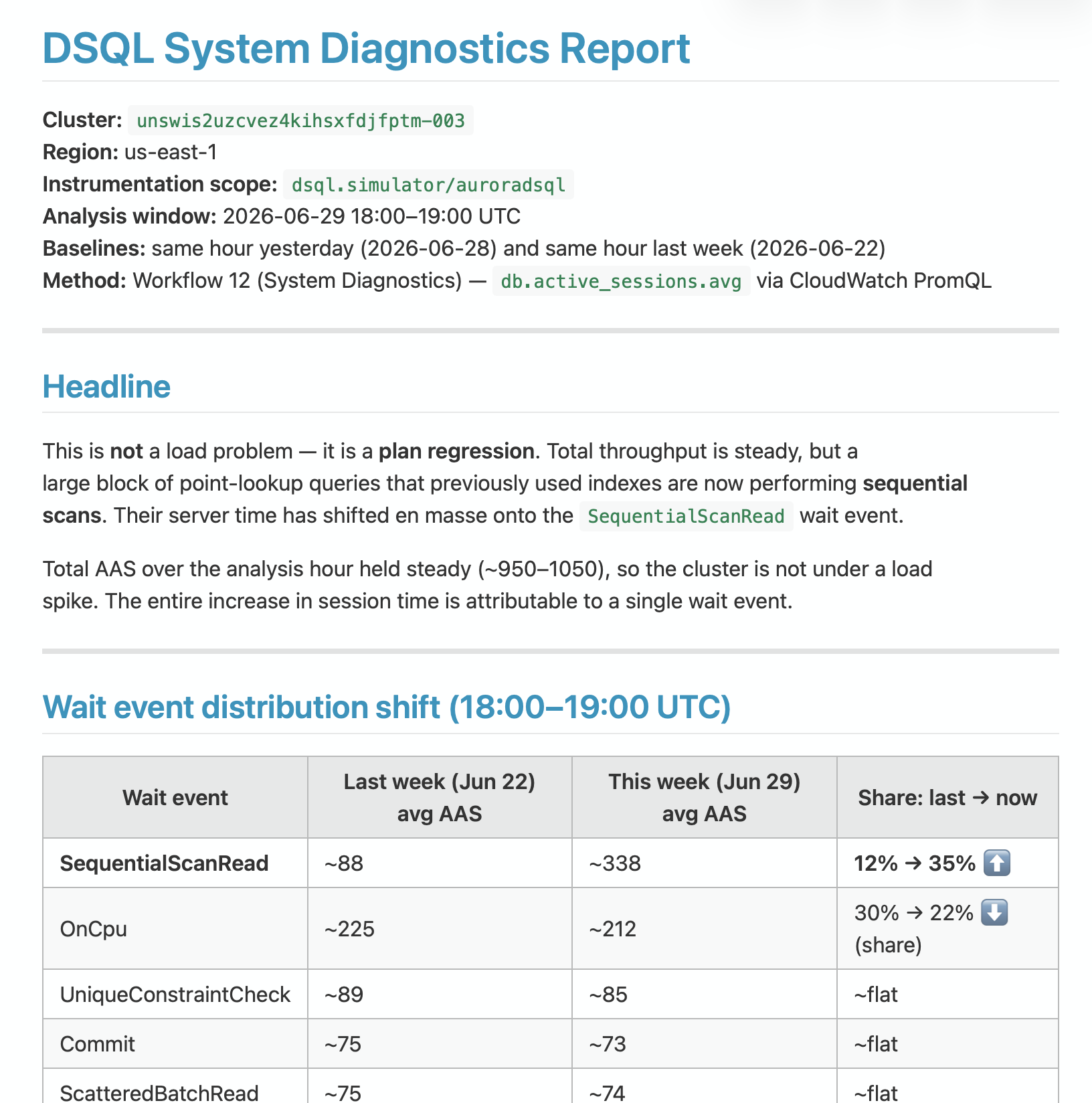
Figure 6: Example Markdown performance report from the DSQL system diagnostics AI skill
Further on in the example report, the report highlights a specific query as a candidate for a poor execution plan:
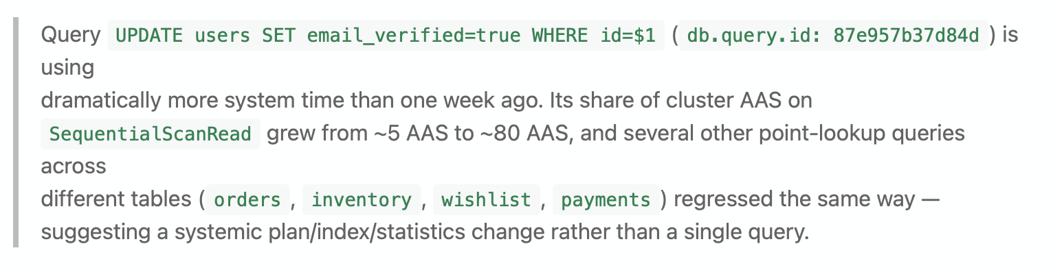
Figure 7: The report highlighting a query that is a candidate for a poor execution plan
If specific queries look problematic, the skill automatically initiates a deep SQL-focused diagnostics workflow and reports diagnostic information for that SQL statement.
Conclusion
The DSQL time-based observability approach gives you a direct, intuitive way to understand where your sessions spend their time, connecting what you observe to both the performance you experience and the costs you incur. Whether you use CloudWatch Database Insights for a visual overview, query DASH data directly with PromQL, or let the DSQL skill handle the analysis, you have the tools to quickly identify bottlenecks, optimize queries, and operate your DSQL clusters with confidence. Try using CloudWatch Database Insights, direct PromQL, or the AI skill to find and fix performance problems quickly in your DSQL cluster.