AWS for Industries
Visualizing Distributed and Edge Applications Performance Using Amazon Quick Suite Sankey Diagram
Introduction
In today’s mission-critical networks, distributed and edge computing plays a vital role in telecommunications, gaming, Edge AI processing, and autonomous vehicles. As distributed applications are deployed across multiple AWS Regions, Availability Zones (AZs), and Local Zones (LZs) to meet customer demands for ultra-low latency services, understanding each node’s performance becomes increasingly complex. Traditional monitoring tools present network data in isolation through time-series graphs showing individual connection metrics, failing to reveal the bigger picture such as bottleneck locations across the entire architecture or how traffic patterns change over time from node to node. As infrastructure scales from a handful to dozens of nodes and locations, analyzing raw metrics becomes overwhelming, making it difficult to identify patterns and make informed planning and expansion decisions.
Amazon Quick Suite’s Sankey diagrams address this challenge by visualizing the flow and relationships between network nodes and locations in a clear and interactive format. This blog post demonstrates how to build a real-time performance visualization pipeline combining EC2 instances running monitoring application, S3 for data storage, AWS Athena for querying, and Amazon Quick Suite for visualization. While latency between nodes is used as the metric in this blog, the solution can expand to visualize other performance metrics such as, bandwidth utilization, application response times, or error rates—adapting to any business need.
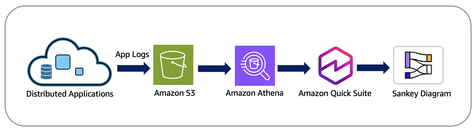
Figure 1: Application logs processing flow through AWS services to Sankey diagram
Implementation Steps
Prerequisites
Before implementing the visualization solution, we established a test environment consisting of 27 EC2 instances across different AWS Regions and Local Zones, running a Python-based monitoring application that continuously measures network latency between all node pairs and stores it in S3.
The Python application stores logs in CSV with the following format in our S3 bucket. However, you could have different fields and format based on your application logs:
| timestamp_utc | timestamp_pdt | protocol | source_ip | source_tag | dest_ip | dest_tag | port | size | rtt |
| 2025-08-22 0:01 | 2025-08-21 17:01 | TCP | 10.0.3.135 | DC_01 | 10.0.8.98 | Edge_01.App02 | 443 | 128 | 13.2 |
This raw data serves as the foundation for our visualization pipeline through Athena and Amazon Quick Suite.
Data Processing with AWS Athena
1. Access Athena
- Open AWS Console (https://console.aws.amazon.com)
- In the search bar at the top, type Athena
- Click on Amazon Athena in the search results
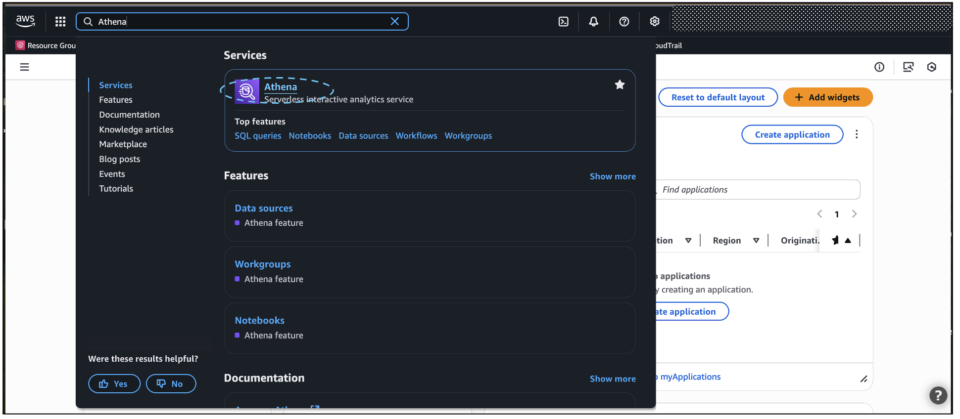
Figure 2: AWS Console – Searching for Athena service
2. Configure Athena Settings (First-time setup)
- If this is your first time using Athena, you’ll see a prompt to configure query results location
- Click on Edit settings
- Enter an S3 bucket path for query results (e.g., s3://your-bucket-name/athena-results/)
- Click Save
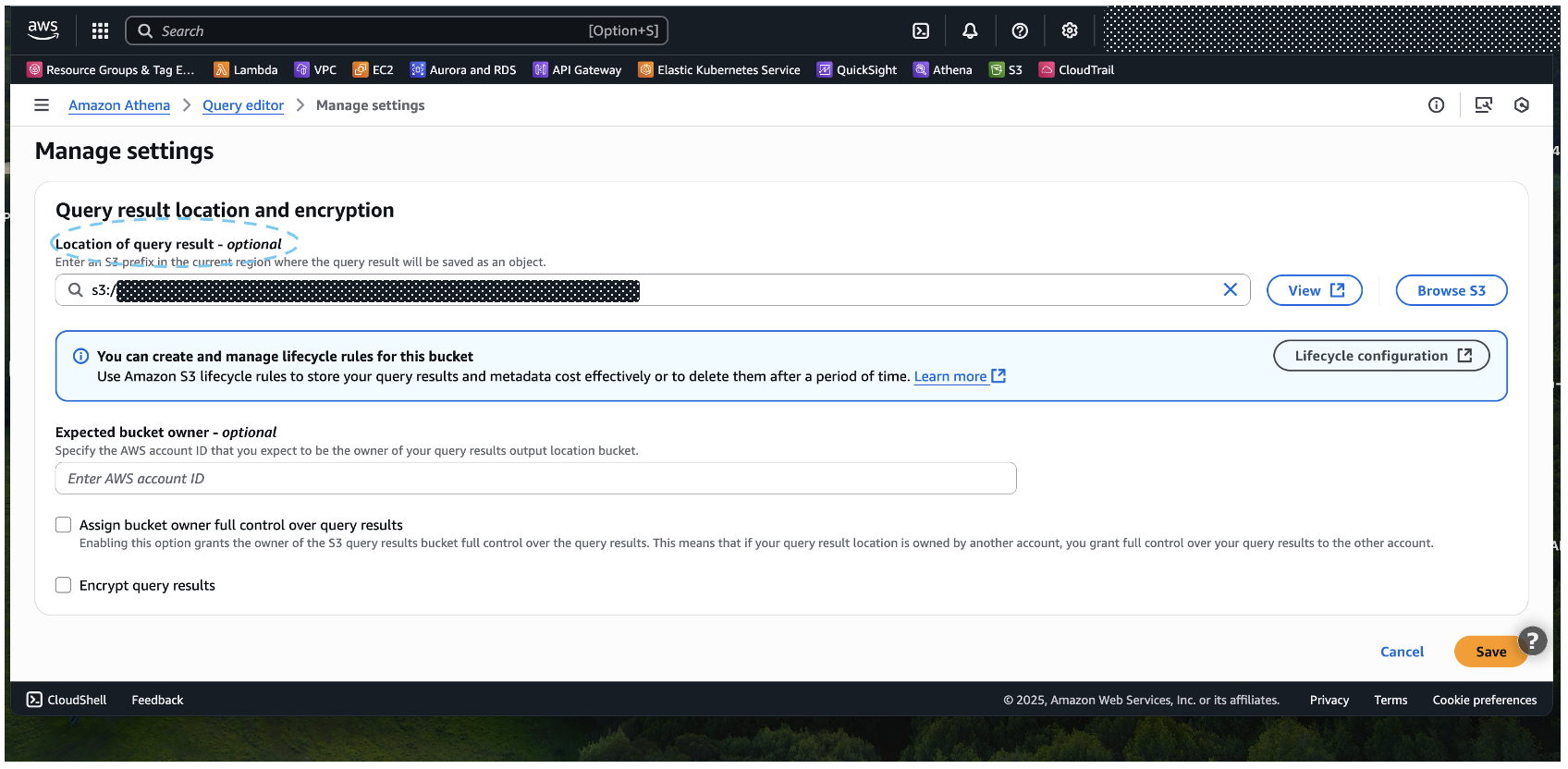
Figure 3: Athena settings – Query result location configuration
3. Create Database
- In the Athena query editor, paste the following query:
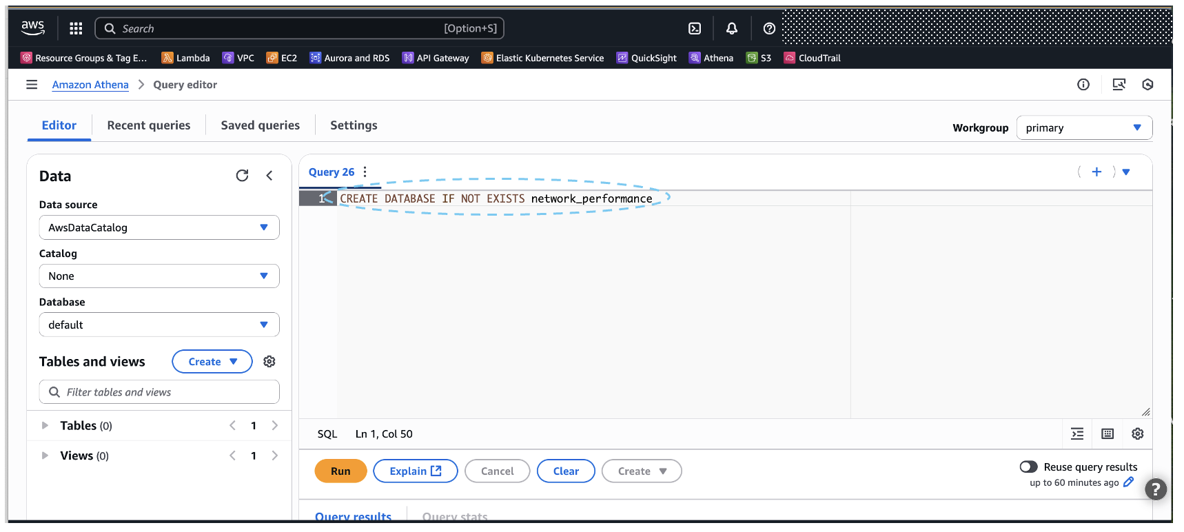
Figure 4: Athena Query editor – Creating network_performance database
- Click Run or press Ctrl+Enter to execute the query
- You should see Query successful message
4. Create Table
- In the database dropdown (left panel), select network_performance
- In the query editor, paste the following query:
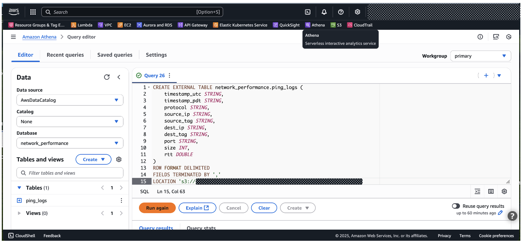
Figure 5: Athena Query editor – Creating ping_logs table schema
- Replace ‘your-bucket-name/path-to-logs/’ with your actual S3 bucket path where the log files are stored
- Click Run to execute the query
5. Verify Table Creation
- In the left panel, click the refresh icon next to Tables
- You should see ping_logs listed under the network_performance database
- Run a test query to verify data access:
Amazon Quick Suite Integration
Configure Athena as Data Source
1. Navigate to Amazon Quick Suite console
2. Select Datasets > Select Data Source > Select Create data source
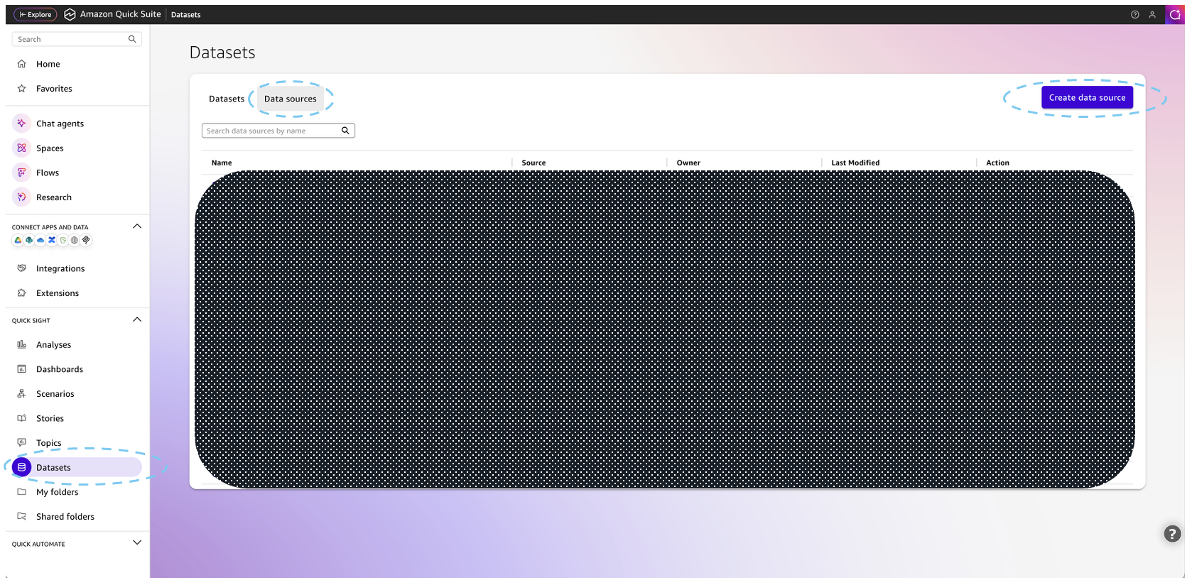
Figure 6: Quick Suite – Data sources
3. Choose Athena as the data source and click Next
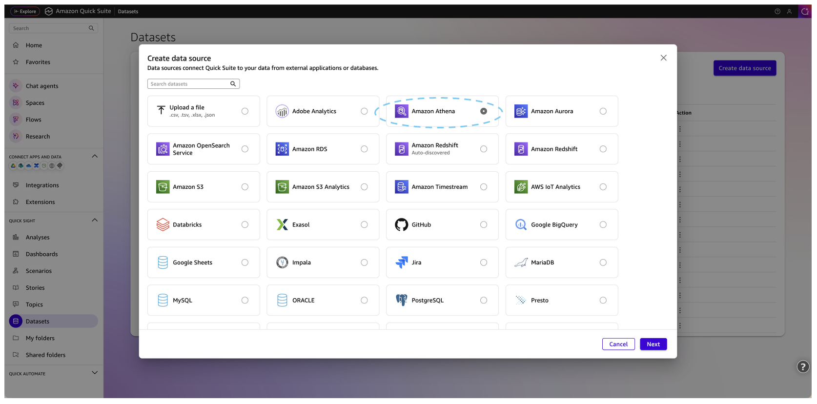
Figure 7: Quick Suite – Selecting Amazon Athena data source
4. Give a name to Data source name and click Create data source.
5. Click on newly created Data Source and click Create dataset
6. Select the network_performance database and ping_logs table
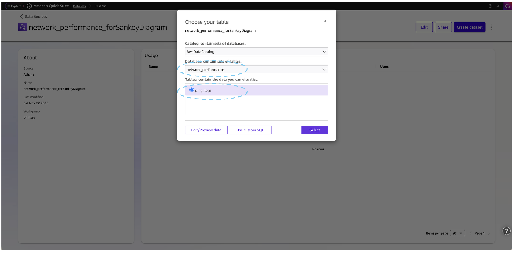
Figure 8: Quick Suite – Choosing ping_logs table
7. Choose Direct query or SPICE based on your needs and follow the prompts
Create Sankey Visualization
1. Add a Sankey diagram visual
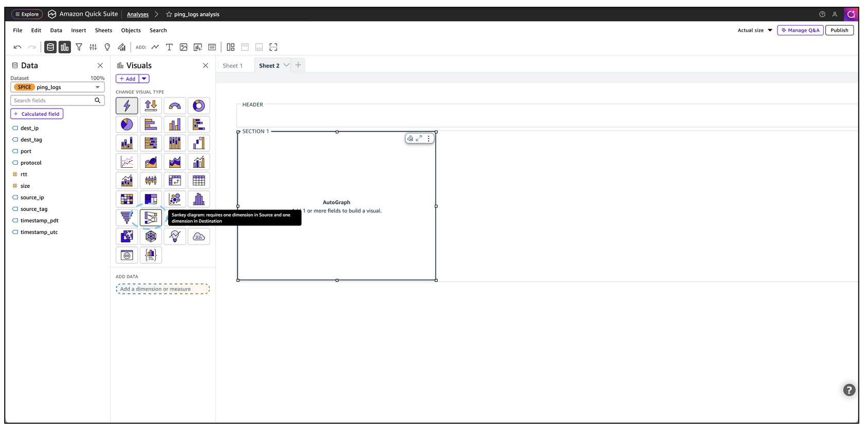
Figure 9: Quick Suite – Selecting Sankey diagram visualization
2. Configure fields:
- Source: source_tag
- Destination: dest_tag
- Weight: rtt (for latency visualization)
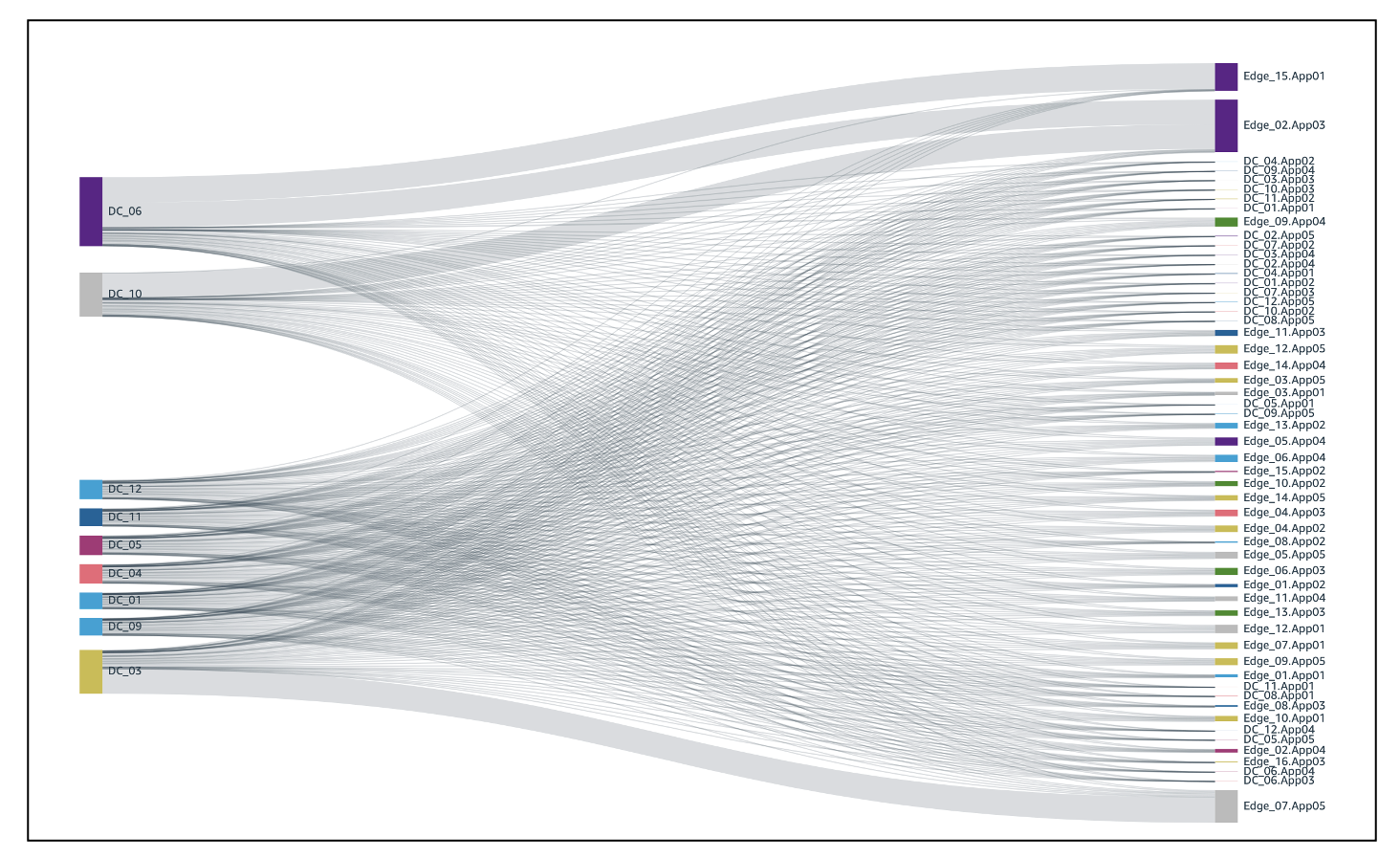
Figure 10: Sankey diagram visualization of network traffic flow
3. Set Up Real-time Refresh
- Double clicks on the recently created Dataset
- Configure appropriate refresh intervals
- Set up error notifications
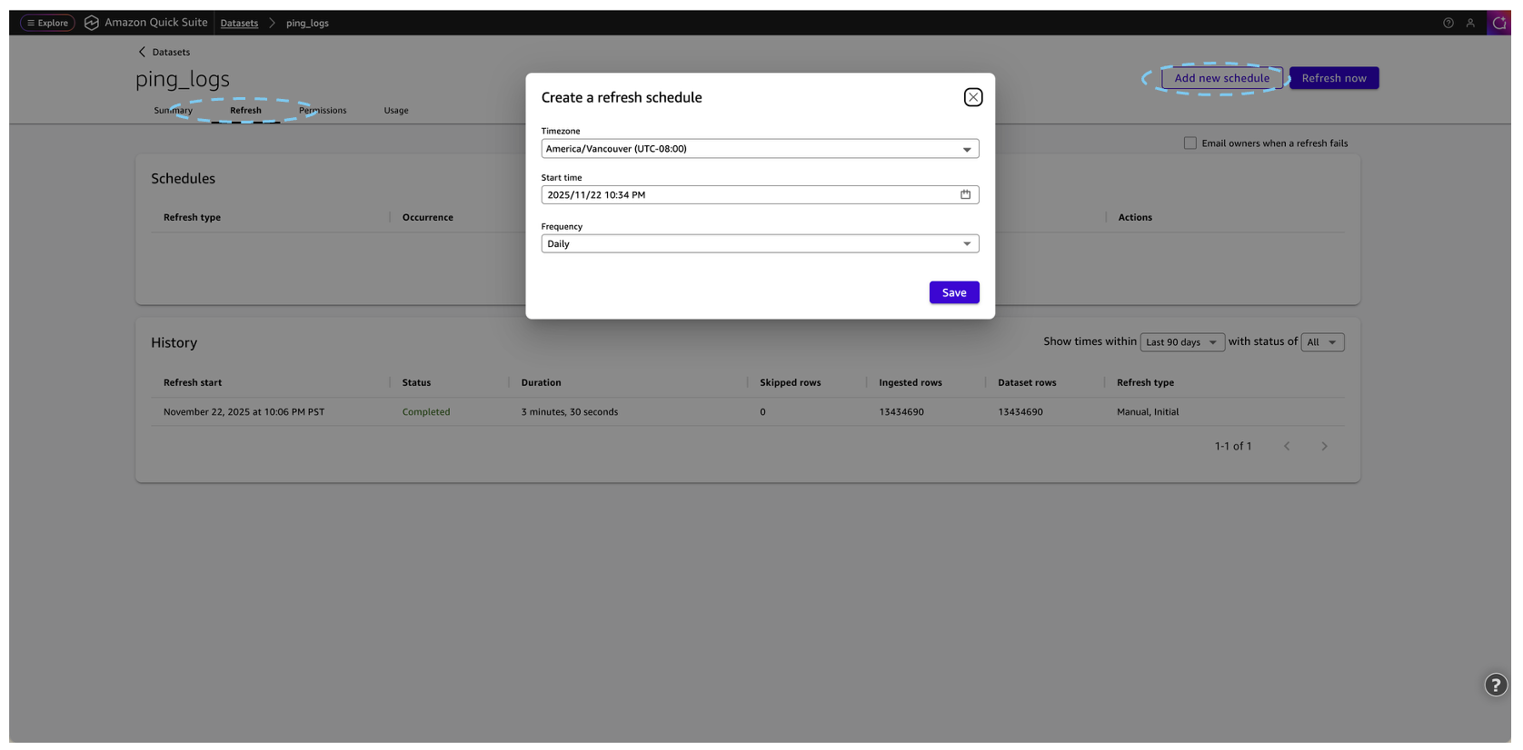
Figure 12: Quick Suite – Refresh Interval
Conclusion
As edge computing continues to grow and distributed architectures become more complex, understanding and optimizing inter-location and inter-node performance is no longer optional but essential for maintaining service quality and competitive advantage. Amazon Quick Suite’s Sankey diagrams transform the overwhelming challenge of monitoring dozens of nodes into an intuitive visual experience that reveals patterns, bottlenecks, and opportunities at a glance. When combined with AWS Athena for querying and S3 for storage, this solution delivers real-time insights into network behavior that enable proactive decision-making and efficient operations. Whether you’re managing a Telco network, gaming platforms, Edge AI processing, or autonomous vehicle networks, this approach provides the visibility needed to optimize performance and plan expansion with confidence.
For telecommunications providers deploying 5G infrastructure, this solution is particularly valuable for monitoring connectivity between Cloud RAN workloads in AWS Local Zones and 5G Core functions in AWS Regions, where understanding network performance and traffic flows are critical for ensuring service quality.
Start visualizing your distributed architecture today and turn complex performance data into actionable intelligence that drives your business forward.
To get started, you can refer to Amazon Quick Suite. To learn more about how CSPs are using AWS, visit Telecom on AWS.