Introducing native histogram support in Amazon Managed Service for Prometheus

If you run Kubernetes or microservices workloads on AWS, you probably track latency, request durations, and other value distributions with Prometheus histograms. To do that with classic histograms, you predefine a set of bucket boundaries, and Prometheus emits one time series per boundary plus a sum and a count. A single latency histogram with 20 buckets becomes 22 active time series. Multiplying that across services, pods, and labels causes histograms to quickly dominate your active series count and inflate cardinality. Worse, you’re still left guessing because your fixed buckets rarely line up with the percentiles you actually care about.

Amazon Managed Service for Prometheus now supports ingestion, storage, and querying of Prometheus native histograms. Native histograms capture an entire distribution in a single time series using exponential bucketing that adapts resolution to your data automatically. DevOps engineers, site reliability engineers, and platform teams get more accurate percentile calculations, far lower cardinality, up to 75% lower metering costs for histogram workloads, and no need to predefine bucket boundaries, all while staying fully compatible with the Prometheus query language you already use.

In this post, you will learn how to:

• Understand how native histograms differ from classic histograms and when to use them
• Send native histograms to your Amazon Managed Service for Prometheus workspace
• Query distributions and tail latency with PromQL using histogram_quantile()
• Confirm the cardinality and cost benefit using Amazon Managed Service for Prometheus vended metrics

Prerequisites

To follow along with this post, you need:

• An active Amazon Managed Service for Prometheus workspace with a remote-write endpoint configured
• A Prometheus client library that supports native histograms (for example, prometheus/client_golang v1.19.0 or later)
• Prometheus server or compatible agent with native histogram support (Prometheus 2.40.0 or later)
• Amazon Managed Grafana workspace (version 10.4 or later) or a Prometheus-compatible query interface for visualization
• AWS Identity and Access Management (IAM) permissions to write metrics to the workspace (AmazonPrometheusRemoteWriteAccess) and read Amazon CloudWatch vended metrics (CloudWatchReadOnlyAccess)

What does this mean for your workspace?

A classic Prometheus histogram divides a value range into a fixed set of buckets that you define ahead of time. Each bucket boundary becomes its own cumulative time series (_bucket), and the histogram also emits _sum and _count series. This design has two costs.

First, every bucket boundary is an active time series, so the bucket count drives your cardinality directly (the 20-bucket, 22-series example from the introduction) before you add a single label.

Second, the accuracy of your percentiles depends entirely on where you placed your buckets. histogram_quantile() cannot see individual observations, only the per-bucket counts, so to estimate a percentile it finds the bucket the value falls into and interpolates linearly, assuming observations are spread evenly across that bucket’s range. When the bucket around your p99 is narrow, that interpolation covers a small range and the estimate stays tight. When the bucket is wide, which is common when your fixed boundaries do not line up with the tail, the interpolation spans a large range of possible values and your tail-latency number can drift away from reality.

Native histograms take a different approach. Instead of fixed boundaries, they use exponential bucketing with a configurable resolution called the schema. The schema is an integer that controls how many buckets cover each factor-of-two range of values (each doubling, also called an octave): a higher schema means more buckets per doubling and finer resolution. Because the layout is defined by a formula rather than by hand-picked boundaries, it adapts to the data automatically. The entire distribution, across all of its populated buckets, is stored as a single time series rather than one series per boundary. The sum and count that classic histograms emit as separate _sum and _count series are embedded within the native histogram sample itself. They are not lost, just no longer separate time series.

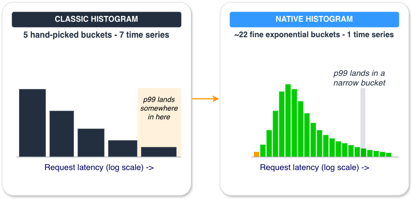
Figure 1. The same latency distribution captured two ways. Classic histograms use a few boundaries you pick in advance, so the tail blurs into one wide bucket. Native histograms lay down a fine exponential ladder automatically, so the tail resolves into a narrow bucket, and the whole distribution is one time series instead of many.

Four things make this significant:

• Lower cardinality. A classic histogram with 20 buckets that previously required 22 time series now requires only one. Native histograms collapse an entire distribution into a single series, which reduces active series count and the cardinality pressure that histograms typically add to a workspace.
• Higher-resolution percentiles. Because resolution adapts to your data instead of relying on hand-picked boundaries, functions like histogram_quantile() return more precise tail-latency insights. You no longer have to predict where your p99 will land when you define the metric.
• Incremental adoption. You can adopt native histograms at your own pace. They run alongside your existing classic histograms, so you can migrate workloads one at a time without disrupting current dashboards or alerts. To migrate: (1) enable native histogram support in your instrumentation (for example, by setting NativeHistogramBucketFactor in the Go client), (2) set scrape_native_histograms: true in your Prometheus scrape configuration so that the scraper collects the native histogram format, and (3) set send_native_histograms: true in your remote_write configuration to forward native histograms to your Amazon Managed Service for Prometheus workspace. Then redeploy. Your application will begin emitting native histograms alongside or instead of classic histograms, depending on your configuration. No changes to your workspace are required.
• Lower cost. Each populated bucket in a native histogram counts as 0.25 of a metric sample, and empty buckets are not metered at all. A histogram with 20 populated buckets is metered as 5 samples rather than 22 separate time series, a 75% reduction in metered volume for the same distribution. You could even double the resolution to 40 buckets and still pay less than half the cost of a 20-bucket classic histogram (40 × 0.25 = 10 metered samples versus 22 series).

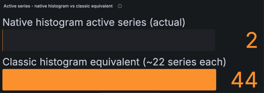
Figure 2. Active series for two latency metrics. As classic histograms they need about 44 series (22 each); as native histograms they need 2 (one each).

How they work

A native histogram represents a distribution of observed values, such as request latencies, by dividing the value range into buckets. Each bucket covers a range of values and holds a count of how many observations fell into that range. The key concept is the difference between populated and empty buckets:

• A populated bucket has a non-zero count of observations. It contains real data points.
• An empty bucket has a count of zero. In a sparse distribution, most of the possible buckets are empty at any given moment.

If a latency histogram has 200 possible buckets but only 20 are typically populated, the distribution you store and query is described by those 20 populated buckets. This sparseness is what keeps native histograms compact and efficient: only populated buckets contribute to the stored distribution, so sparse distributions stay lightweight.

The following figure shows a real native histogram queried back from an Amazon Managed Service for Prometheus workspace. It is a single request_latency_seconds time series, yet it describes the full latency distribution across its populated exponential buckets.

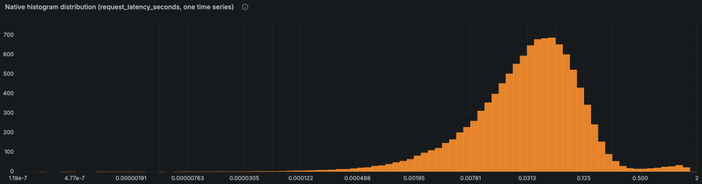
Figure 3. A native histogram distribution (request_latency_seconds) queried from a workspace and visualized in Grafana. The horizontal axis is latency and the vertical axis is observation count. The full distribution is stored as one time series.

How do classic and native bucket counts compare during migration?

Classic and native histogram bucket counts are not equivalent, so it helps to know what to expect before you migrate. Suppose you have a classic histogram with 11 buckets and you switch to native histograms using the default settings (NativeHistogramBucketFactor: 1.1, which corresponds to schema 3). You will not get 11 buckets back; you will get roughly 80.

As described earlier, the schema sets how many buckets cover each doubling of the value range. Schema 3 uses eight buckets per doubling. A typical latency range runs from about 0.125s to 128s, which is roughly 10 doublings. Eight buckets per doubling across 10 doublings gives a maximum of about 80 bucket positions. Remember that only populated buckets are ever stored and metered, so the actual number you pay for is usually much lower.

If 80 is more resolution than you need, you have two levers. Set NativeHistogramMaxBucketNumber to cap the bucket count, and the client automatically reduces resolution to stay within the limit. Or increase NativeHistogramBucketFactor (for example, from 1.1 to 1.5) to use a coarser schema with fewer buckets per doubling. Either way, native histograms remain more cost-effective, because each populated bucket is metered at 0.25 of a metric sample. Even 80 populated native histogram buckets cost the equivalent of 20 metric samples, comparable to a single classic histogram with 20 buckets (22 series).

Sending data to your workspace

Native histograms are produced by your instrumentation, not by a configuration change in the workspace. Any Prometheus client library that supports native histograms can emit them, and any collector or remote-write pipeline that already sends metrics to Amazon Managed Service for Prometheus can carry them.

For example, with the Go client library you enable native histogram buckets by setting a bucket factor when you create the histogram:

import "github.com/prometheus/client_golang/prometheus"

// NativeHistogramBucketFactor enables a native histogram.
// A factor of 1.1 gives roughly 10% resolution between buckets.
latencySeconds := prometheus.NewHistogramVec(prometheus.HistogramOpts{
	Name:                           "request_latency_seconds",
	Help:                           "Request latency distribution (native histogram).",
	NativeHistogramBucketFactor:    1.1,
	NativeHistogramMaxBucketNumber: 160,
}, []string{"service"})

Point your collector or agent at your workspace’s remote-write endpoint as you do today. No workspace configuration change is required to ingest native histograms.

Query distributions with PromQL

Native histograms work with the same PromQL you already use, with one quality-of-life difference: you query the metric directly instead of the per-bucket _bucket series. To calculate p99 latency from a native histogram, pass the metric to histogram_quantile():

# p99 request latency from a native histogram, per service
histogram_quantile(0.99, sum by (service) (rate(request_latency_seconds[5m])))

Run against a workspace, this returns one value per service, reading from the single native histogram series. Each result is a [timestamp, value] pair, where the value is the p99 latency in seconds:

{ "resultType": "vector", "result": [
  { "metric": { "service": "checkout" }, "value": [ 1780772294, "0.738" ] },
  { "metric": { "service": "search"   }, "value": [ 1780772294, "0.866" ] }
] }

Compare that to the classic-histogram form, which has to aggregate the explicit le (less-than-or-equal) bucket label:

# p99 from a classic histogram requires aggregating the _bucket series by le
histogram_quantile(0.99, sum by (service, le) (rate(request_latency_seconds_bucket[5m])))

Both queries return a p99, but the native histogram version reads from a single series and adapts its resolution to your data, so the result is more precise at the tail. You can run these queries from your Amazon Managed Grafana workspace or any Prometheus-compatible query interface pointed at your workspace.

Note: Native histogram visualization in Amazon Managed Grafana requires workspace version 10.4 or later. If your workspace is on an earlier version, upgrade it to visualize native histogram distributions natively.

Confirm cardinality and cost benefits with vended metrics

You can confirm the cardinality benefit, and understand cost attribution, using the Amazon Managed Service for Prometheus vended metrics in Amazon CloudWatch. The following figure shows ActiveSeries for the whole workspace alongside NativeHistogramActiveSeries: the native histograms account for only a couple of series while still carrying full distributions.

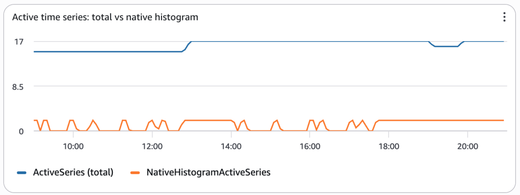
Figure 4. Amazon CloudWatch vended metrics for the workspace. NativeHistogramActiveSeries stays low because each distribution is a single series.

Monitoring costs

If you ingest native histograms, you can use the following vended CloudWatch metrics to monitor cost drivers and usage:

• NativeHistogramIngestedBucketsRate – Monitors the rate of populated buckets being ingested. Because native histograms are metered based on populated buckets, this metric provides direct visibility into your native histogram cost drivers.
• NativeHistogramIngestionRate – Tracks the overall native histogram sample ingestion rate into your workspace.
• NativeHistogramActiveSeries – Monitors the number of active native histogram series in your workspace.

These metrics help you understand exactly how much of your workspace’s metered volume comes from native histogram workloads, making it straightforward to attribute costs and plan capacity.

Pricing

Native histogram support is available at standard Amazon Managed Service for Prometheus rates, with no new pricing dimension to manage. Native histogram metered samples are priced at the same per-sample rate as regular metric samples and count toward the same volume tiers. The one difference is how samples are counted: each populated bucket (a bucket with non-zero observations) counts as 0.25 of a metric sample, and empty buckets are not metered. For example, a native histogram with 10 populated buckets is metered as 2.5 metric samples. As shown earlier, this works out to up to a 75% reduction in metered volume compared to equivalent classic histogram series. For full pricing details, see the pricing page.

Cleaning up

If you enabled native histograms for testing and want to stop ingestion to avoid ongoing charges, follow these steps:

1. Remove native histogram configuration from your instrumentation. Remove or comment out the NativeHistogramBucketFactor setting from your histogram definitions.
2. Redeploy your application. The application will revert to emitting only classic histograms (or no histograms, depending on your configuration).
3. Set scrape_native_histograms: false in your Prometheus scrape configuration to disable native histogram collection.
4. Set send_native_histograms: false in your remote_write configuration to disable native histogram forwarding.
5. Reload or restart your Prometheus server or agent to apply the configuration changes.
6. (Optional) Delete your Amazon Managed Service for Prometheus workspace. If you created a workspace specifically for this walkthrough and no longer need it, in the Amazon Managed Service for Prometheus console, delete the workspace. Note that this permanently deletes all metrics data in the workspace.
7. (Optional) Delete your Amazon Managed Grafana workspace. If you created a workspace specifically for this walkthrough and no longer need it, in the Amazon Managed Grafana console, delete the workspace. Note that this permanently deletes all dashboards, data sources, and configuration in the workspace.

Stopping ingestion prevents future metering charges. Existing data continues to count toward storage until it expires according to your workspace retention policy.

Conclusion

This post introduced Prometheus native histogram support in Amazon Managed Service for Prometheus: how native histograms collapse a full distribution into a single time series, how to emit and query them with the PromQL you already use, and how they reduce both cardinality and metered volume by up to 75% for histogram workloads.

With native histograms, you get higher-resolution tail-latency insights, lower cardinality, and significant cost savings without predefining bucket boundaries or managing one series per bucket. Amazon Managed Service for Prometheus continues to reduce the operational cost of running Prometheus at scale while improving the accuracy of your metrics.

Native histogram support is available in all AWS Regions where Amazon Managed Service for Prometheus is offered. To get started, emit native histograms from your instrumentation and send them to your workspace, then query them in Amazon Managed Grafana or any Prometheus-compatible interface.

For more on instrumenting and operating Prometheus on AWS, explore the following resources:

• Amazon Managed Service for Prometheus documentation: setup, collector configuration, and querying
• Amazon Managed Service for Prometheus pricing: pricing details for Amazon Managed Service for Prometheus
• Prometheus native histograms documentation: the open-source specification and client library support