AWS Open Source Blog
Unified Knowledge Graph RAG on AWS: GraphRAG and LightRAG on one stack
Picture a compliance analyst staring at a few thousand contracts, amendments, and internal memos, trying to answer one question that sounds straightforward: “Which of our obligations are exposed if this one milestone slips?” The answer isn’t written in any single document. It’s stitched across three — a master agreement that ties a payment to a milestone, an amendment that reschedules that milestone, and a risk memo that traces the knock-on effect down the supply chain. A keyword search returns the paragraphs that mention “milestone”; it can’t follow the thread between them.
If you’ve built a Retrieval-augmented generation (RAG) system, you already know why. RAG enables you to embed your documents, retrieve the chunks nearest a question, and then let the model answer from them. The RAG approach shines when the answer sits in one passage you can find by similarity. It strains when the answer is spread across many documents, or lives in the relationships between entities rather than in the words themselves. Our analyst’s question is exactly that shape: “what depends on what” is a structure in the data, not a paragraph you can retrieve. Knowledge-graph RAG is built for this. It first turns a corpus into a graph of entities and their relationships, then reasons over that structure instead of over isolated chunks.
That is what unified-kg-rag-on-aws (Apache-2.0) is for. It brings two knowledge-graph RAG methodologies — Microsoft’s GraphRAG and HKUDS’s LightRAG — onto one shared stack built on Amazon Bedrock, Amazon Neptune, and Amazon OpenSearch Service. You choose the retrieval methodology per query, and everything underneath — ingestion, indexing, caching, multilingual handling — is shared. The rest of this post walks through the problem it solves, the two methodologies it builds on, what it adds, how the whole thing fits together end to end, and what it scores when measured against public benchmarks and against the reference implementations themselves.
Where vector search runs out of road
Vector-only RAG retrieves by embedding similarity, so it judges each chunk in isolation. That is fine for “What is the warranty period in section 4?” but it struggles with questions whose answers are distributed or relational:
- Multi-hop. “Which obligations depend on a milestone that this amendment changed?” The reasoning chain spans documents that never share embedding-similar wording.
- Cross-document aggregation. “Which clauses across all contracts reference the same indemnity cap?” No single chunk contains the answer.
- Global / thematic. “Summarize the main themes and risks across the entire corpus.” There is no “nearest chunk”; the answer is a synthesis over everything.
Top-k nearest-neighbor retrieval returns locally similar text, not the connective structure that actually answers these questions. That structure is exactly what a knowledge graph captures.
Two ideas we build on: GraphRAG and LightRAG
Two open source methodologies shaped this space, and this project re-implements both from their papers (clean-room; no upstream code was copied — attribution lives in THIRD_PARTY_LICENSES).
Microsoft GraphRAG — community summarization (arXiv:2404.16130, GitHub). GraphRAG’s central bet is to spend the expensive reasoning once, at indexing time, so that queries stay cheap.
During ingestion, an LLM reads the corpus and extracts an entity-and-relationship graph: Acme Corp, Milestone 3, the indemnity clause, and the edges between them. Then Leiden community detection looks for clumps in that graph — sets of entities that reference each other far more than they reference anything else. Those clumps are the “communities”, and they are worth pausing on, because nobody chose them. They are not your folder structure or your document tags; they are topics that fall out of how the corpus actually hangs together. A contract, its amendment, and the risk memo that traces the knock-on effect will land in one community even if they live in three different systems.
An LLM then writes a summary of each community, and of each cluster of communities above it, producing a tree of thematic summaries — your corpus, pre-digested at several zoom levels. That tree is what makes two different kinds of question answerable:
- A global question (“what are the major risks across everything?”) never touches the raw documents. It fans out across the community summaries, answers from each, and reduces those partial answers into one — map-reduce over topics.
- A local question (“what does the corpus say about Milestone 3?”) starts from the entities the question names, then walks outward along their relationships, collecting the neighbors and the text behind them.
Building that tree costs real money at ingestion time, and querying it costs again — the benchmarks later in this post put numbers on both, and the results are not what the framing predicts. This project exposes GraphRAG as the simple, local, global, drift, and auto strategies (auto lets an LLM router pick per query).
LightRAG — dual-level keyword retrieval (arXiv:2410.05779, GitHub). LightRAG takes the opposite bet: keep indexing cheap and do the thinking when the question arrives. It still extracts an entity-and-relationship graph, but it stops there — no community detection, no summaries.
The interesting part happens at query time. Given a question, LightRAG pulls out two kinds of keyword and sends each to a different layer of the graph. Take “which of our obligations are exposed if this milestone slips?”:
- Low-level keywords name the concrete things — obligation, milestone. These are matched against entity descriptions: the “what things are” layer.
- High-level keywords capture what the question is really getting at — exposure, dependency, schedule risk. These are matched against relationship descriptions: the “how things connect” layer.
Searching both layers in one pass is what gives it breadth and precision together. The entity layer keeps the answer anchored to real things in your corpus; the relationship layer surfaces the connections you didn’t name, which is where a multi-hop answer usually hides. And because there is no summarization step, you can point it at a corpus and start asking questions sooner.
The trade-off is that the work moves to every query rather than being paid once, and the benchmarks later show LightRAG’s modes carrying the highest per-query cost of any strategy that competes on accuracy — “lightweight” describes the indexing, not the retrieval. This project exposes LightRAG as the mix, hybrid, and naive strategies.
What we added on top
The two methodologies make opposite bets, and which bet is right depends on questions you may not be able to answer before you have a corpus indexed. Rather than force that choice up front, this framework makes both interchangeable over shared infrastructure. Five deliberate additions sit on top of the papers:
- Two methodologies, one stack. Set
RAGInput.search_strategyper query to switch between GraphRAG (simple/local/global/drift/auto) and LightRAG (mix/hybrid/naive) — over the same ingested graph, indices, and cache. - Triple-hybrid retrieval. Every query fuses lexical, semantic, and graph retrieval into one ranked context instead of relying on embedding similarity alone.
- Incremental indexing. Re-runs re-index only new or changed documents, so adding to a corpus does not mean re-paying for the whole thing. Changing the extraction prompts or the chunking config still requires a rebuild, since those alter what every document would produce.
- Multilingual by design. A dedicated translation stage, language-aware analyzers, and multilingual keyword/entity extraction apply under both methodologies.
- Hexagonal architecture. The domain/ layer has no boto3 or LangChain imports. Retrieval strategies self-register through a decorator, storage backends are injected as constructor arguments, and evaluators and renderers resolve through their own type-to-class maps — so swapping a backend or adding a strategy is an additive change rather than an edit to dispatch code.
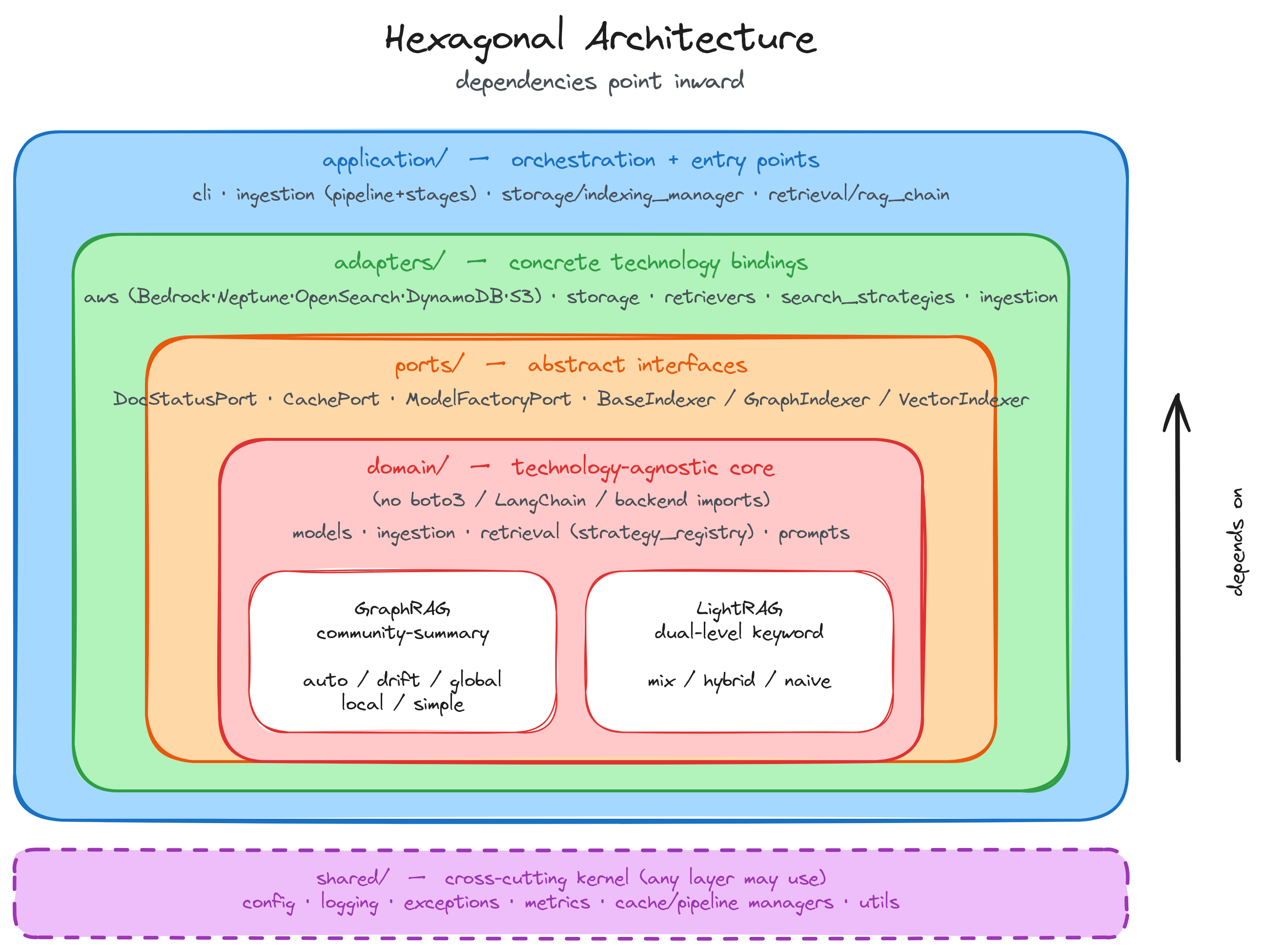
Hexagonal layers: a technology-agnostic domain core wrapped by adapters that bind to Bedrock, Neptune, and OpenSearch through registries.
Following a corpus through the system
Let’s trace a corpus end to end: raw files, ingestion, retrieval, the AWS services behind each step, and how to run it yourself.
Ingestion: from raw documents to a knowledge graph
Ingestion is a checkpointed, resumable pipeline of 12 stages (pipeline.py). Grouped into phases:
1. Prepare → document_parsing, document_loading, text_chunking, translation. Files are parsed (pluggable loaders), loaded, chunked, and — if configured — translated to a target language for consistent extraction.
2. Build the graph → graph_extraction, gleaning, graph_resolution, claim_extraction, claim_resolution. An LLM extracts entities and relationships per chunk; gleaning re-prompts to catch missed items; graph_resolution merges duplicate/co-referent entities; claims (factual assertions with provenance) are extracted and resolved.
3. Analyze & index → graph_analysis, community_detection, indexing. Graph metrics are computed, Leiden community detection groups entities and generates hierarchical community summaries, and the pipeline writes everything into Neptune (graph) and OpenSearch (lexical + vector indices).
Each stage checkpoints to a local cache (optionally synced to Amazon Simple Storage Service (Amazon S3)), so a run resumes from the last completed stage with --pipeline-id and --resume-from-stage.
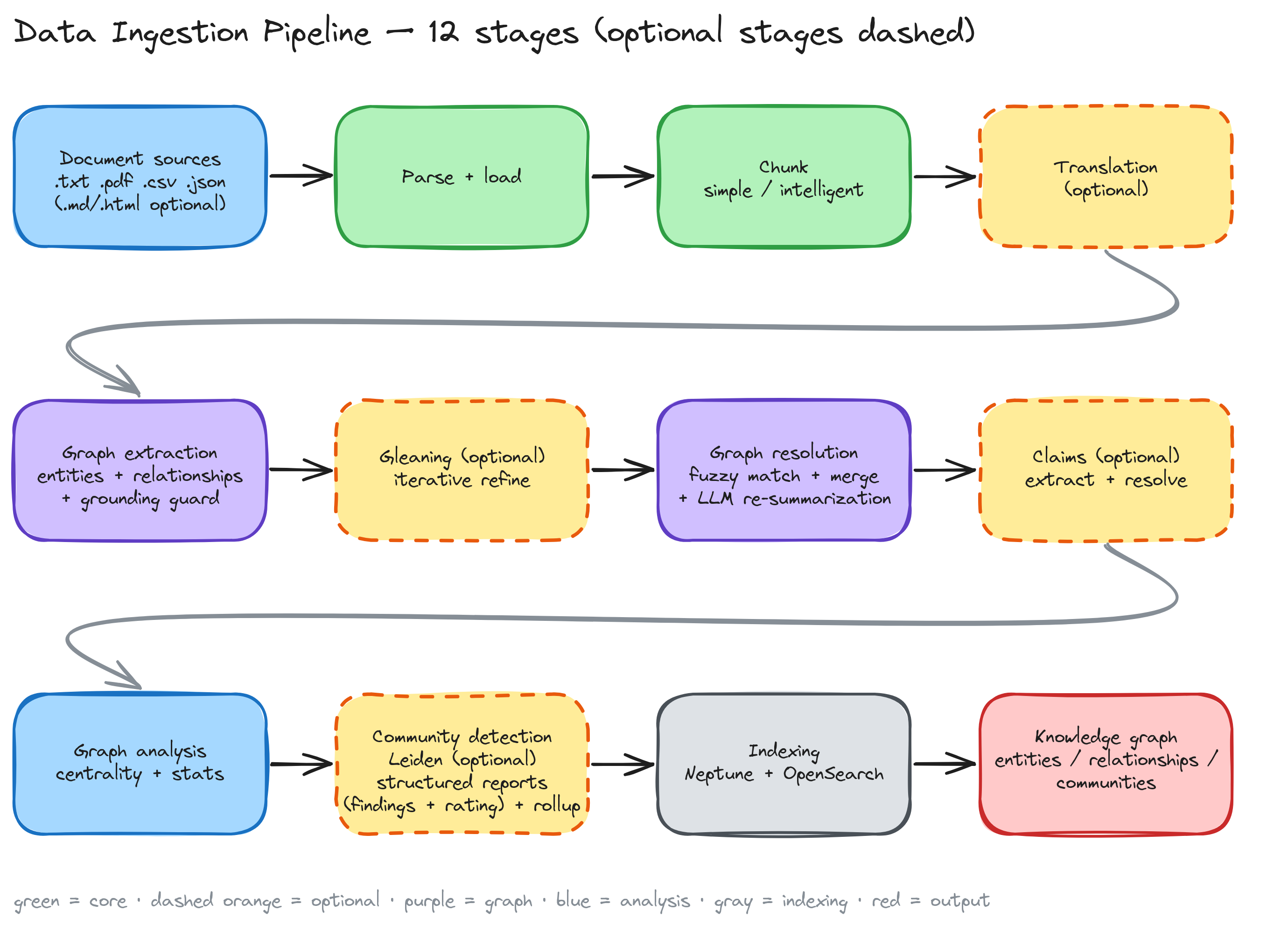
The 12-stage pipeline, from document parsing through community detection to indexing; every stage is a resumable checkpoint.
Re-indexing only what changed
Enable the Amazon DynamoDB registry (add aws.dynamodb to config) and each document’s content hash is recorded (incremental.py). On the next run, unchanged documents are skipped, new or changed documents are re-extracted, and their artifacts are merged into the live graph via idempotent upserts. Because the registry tracks per-document lineage, deleting a document removes only the graph/index artifacts exclusive to it — shared entities survive.
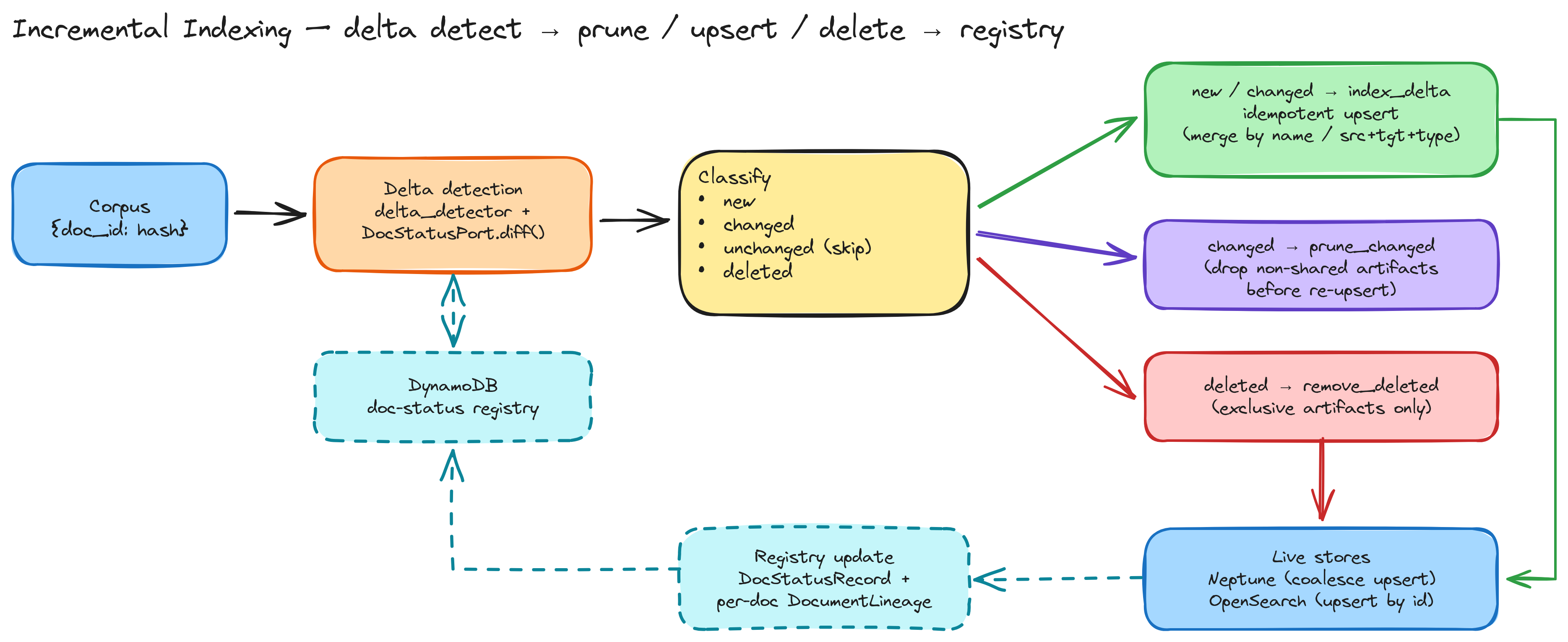
A content-hash delta skips unchanged documents and merges only new or changed artifacts, with per-document lineage driving exclusive-artifact deletion.
Answering a query: three retrievers, one backbone
Triple-hybrid retrieval runs on every query as a fixed backbone; the selected strategy only changes how the graph is traversed. A query flows through:
- Process the query — optional translation plus high/low keyword and entity extraction.
- Retrieve from three stores — OpenSearch BM25 (lexical), OpenSearch kNN over Bedrock embeddings (semantic), and Neptune graph expansion (structural).
- RRF-fuse the three ranked lists with Reciprocal Rank Fusion (
hybrid_scorer.py). - Optional Bedrock rerank of the fused list.
- Assemble a token-budgeted context.
- Generate a grounded answer with source attributions.
This is where the strategy choice pays off, and it maps back to the three question types we started with. A global / thematic question can use GraphRAG global, running map-reduce over community summaries to synthesize across the whole corpus. A multi-hop question can use local entity expansion to follow the chain of relationships from one document to the next. An entity-centric question can use LightRAG mix, retrieving by dual-level keywords. Only the graph traversal changes; the fusion, rerank, and generation steps underneath stay identical — which is what makes switching cheap enough to test empirically rather than reason about. The benchmarks later in this post do exactly that, and one of those three pairings does not survive the measurement.
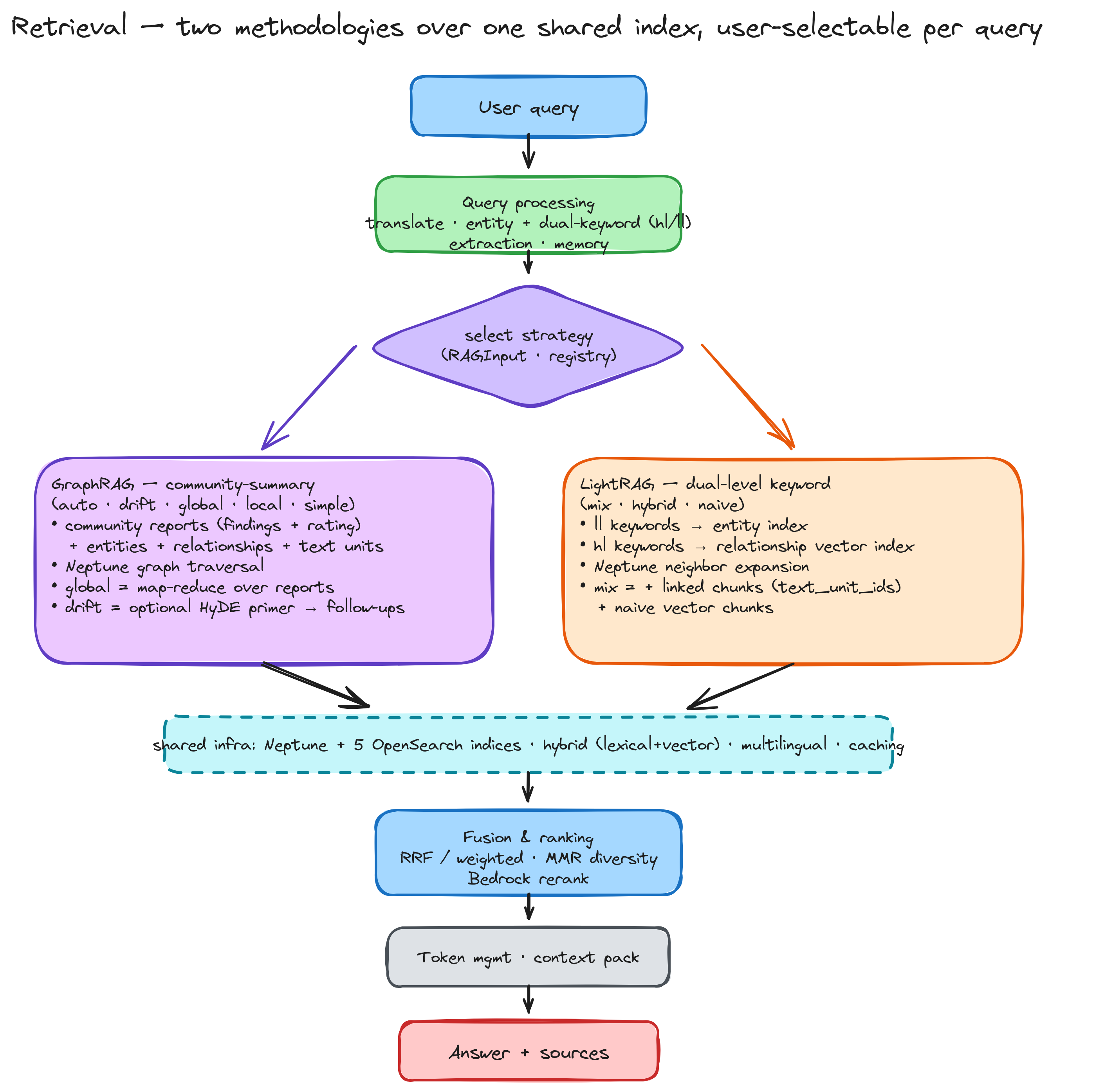
One retrieval backbone — three retrievers fused by RRF, an optional rerank, then grounded generation — with the chosen strategy deciding only how the graph is traversed.
Which AWS service does what
Each concern maps onto a managed AWS service:
| Concern | AWS service | How it’s used |
|---|---|---|
| LLMs, embeddings, rerank | Amazon Bedrock | Extraction/summarization/generation, embeddings for kNN, optional rerank. Cross-region inference profiles and prompt caching are applied per model, since both depend on the model supporting them |
| Graph store | Amazon Neptune | Entity/relationship graph, idempotent fold/coalesce upserts. Access is via Gremlin only — Neptune also speaks openCypher, but this project does not use it |
| Lexical + vector search | Amazon OpenSearch Service | A BM25 text index plus a kNN vector index (Lucene engine, cosine similarity). Works against a managed domain or a Serverless collection |
| Incremental state | Amazon DynamoDB | Optional doc-status registry: content-hash delta + per-document lineage |
| Corpus + cache | Amazon S3 | Source documents and resumable pipeline cache |
Running it yourself
Start with the Quickstart to go clone → ingest → query, then drop into Python for programmatic use.
Before you start: this project is a reference implementation and sample, not production-ready as-is. It provisions real Neptune, OpenSearch, and Bedrock capacity, so review security, cost, scaling, and data-governance settings for your environment before any production use.
git clone https://github.com/awslabs/unified-kg-rag-on-aws.git
cd unified-kg-rag-on-aws
uv sync --extra dev

# Set the Bedrock model IDs, Neptune and OpenSearch endpoints, S3 buckets,
# and AWS region; add an aws.dynamodb section to enable incremental indexing.
cp config-template.yaml config.yaml

# Ingest a corpus (resumable - re-run with --resume-from-stage after a failure)
run-ingestion --source-directory ./source --s3-sync --s3-bucket-name my-bucket

# Query, switching methodology with --search-strategy
run-rag --query "Summarize the key risks across the corpus." --search-strategy global
run-rag --query "What entities relate to the indemnity cap?" --search-strategy mix

# Also available
run-eval             # langchain / ragas / graph-aware evaluators
run-visualization    # render an exported graph, no ingestion
run-prompt-tuning    # profile a corpus -> domain-adapted prompts
Prerequisites: Python 3.11+, uv, configured AWS credentials, and a Bedrock account with the models enabled in your region.
If your corpus is domain-specific — legal, medical, financial — it’s worth running run-prompt-tuning first. It samples the corpus, infers the domain, language, and entity types, and writes tuned extraction prompts you can drop into your config before ingesting. It’s optional, and its effect is not part of the benchmarks below — those ran without it, on general-domain corpora.
You can also drive the same flow from Python, which is handy when you’re embedding the framework in a larger service:
import asyncio
from unified_kg_rag.shared import get_config
from unified_kg_rag.application.retrieval.rag_chain import (
    create_rag_chain, RAGInput,
)
from unified_kg_rag.domain.models import SearchStrategy

async def main():
    config = get_config("config.yaml")
    chain = await create_rag_chain(config=config)
    try:
        # GraphRAG global; swap to SearchStrategy.MIX for LightRAG
        result = await chain.ainvoke(RAGInput(
            query="Which obligations depend on a milestone the amendment changed?",
            search_strategy=SearchStrategy.GLOBAL,
            top_k=10,
        ))
        print(result.answer)
        for src in result.sources:
            print(src)

        # Same graph, LightRAG dual-level keyword retrieval:
        lightrag_result = await chain.ainvoke(RAGInput(
            query="What entities relate to the indemnity cap?",
            search_strategy=SearchStrategy.MIX,
            top_k=10,
        ))
        print(lightrag_result.answer)
    finally:
        await chain.aclose()

asyncio.run(main())
To deploy the infrastructure, the optional AWS CDK app in iac/ provisions the full stack — VPC with endpoints, Neptune, OpenSearch, DynamoDB, S3, an ECS Fargate data plane, and a Step Functions state machine that runs the ingestion pipeline as resumable phases — with Well-Architected defaults (private VPC, KMS encryption, TLS, least-privilege IAM) and an optional Bedrock Guardrail.
The CDK app provisions a provisioned-capacity Neptune cluster and an OpenSearch managed domain; adapt the stack if you would rather run Serverless variants. As noted above, treat all of it as a starting point rather than a production deployment.
Adding your own strategy or backend
Adding a retrieval strategy never touches a central if/elif. Strategies self-register into the strategy registry and declare which retriever roles they need; the composition root binds each role to a concrete backend. Implement the abstract asearch method and register under a SearchStrategy enum member (the members below are illustrative placeholders):
from unified_kg_rag.domain.retrieval.strategy_registry import register_strategy
from unified_kg_rag.domain.models import (
    SearchStrategy, RetrieverRole, SearchQuery, SearchResult,
)
from unified_kg_rag.adapters.retrieval.base import BaseSearchStrategy

@register_strategy(SearchStrategy.MY_STRATEGY, required_roles=(RetrieverRole.GRAPH,))
class MyCustomStrategy(BaseSearchStrategy):
    async def asearch(self, query: SearchQuery) -> SearchResult:
        ...
Storage backends follow the same additive principle by a different route: inject them as constructor arguments (IndexingManager(vector_indexer=…, graph_indexer=…)) rather than registering them. Evaluators and visualization renderers each resolve through their own type-to-class map. For a worked example of a strategy, see lightrag_search.py, which implements the dual-level keyword retrieval described earlier.
Which strategy should you reach for?
Eight strategies is a lot of choice, and the papers behind them don’t tell you which one fits your corpus. So we measured — on the multi-hop questions this post opened with, since that is where a graph is supposed to earn its keep, and against the reference implementations rather than only against each other.
The setup: two public benchmarks, MuSiQue and 2WikiMultihopQA, 100 questions each, built so no single document holds the answer. Every strategy answers the same questions over the same graph with the same model, graded by the same scorer. Scores are token-F1 (1.0 matches the reference exactly, 0.0 not at all), each the mean of three runs.
One caveat to carry throughout: these are results on these benchmarks, not universal rankings. Both were designed to need hops between documents, so they flatter graph retrieval by construction. Even across just these two datasets the order changed. Expect your own corpus to reshuffle it again.
Does it behave like the originals?
Since this framework re-implements both methodologies, the first thing to check is whether those re-implementations are faithful — an approximation that scores well is still the wrong tool if you chose it expecting the paper. Both upstream projects were installed, pointed at the same corpus and questions, and scored by the same offline scorer, so the only thing differing between a row’s two columns is the retrieval implementation.
| strategy | this framework | upstream | difference |
|---|---|---|---|
| LightRAG mix | 0.602 / 0.654 | 0.591 / 0.629 | +0.01 / +0.03 |
| LightRAG hybrid | 0.634 / 0.628 | 0.567 / 0.629 | +0.07 / −0.00 |
| LightRAG naive | 0.354 / 0.424 | 0.319 / 0.430 | +0.03 / −0.01 |
| GraphRAG local | 0.519 / 0.577 | 0.404 / 0.471 | +0.12 / +0.11 |
Each cell reads MuSiQue / 2Wiki. simple has no upstream counterpart. GraphRAG global and drift are omitted because both answer from community summaries rather than documents, and these benchmarks ask for single named values that a summary is written by discarding — neither implementation can answer them. global is judged on its own terms below.
Every LightRAG difference above sits inside statistical noise — a paired bootstrap on the per-question scores puts zero inside every confidence interval. That is the headline: pick mix and you get the retrieval behavior the paper describes, not a loose approximation of it.
GraphRAG’s local is the one genuine improvement, and the reason is what each implementation puts in front of the model. Upstream favors the graph’s own one-line descriptions; this framework carries the underlying document passages with them, so full passages make up 17% of its context against upstream’s 4%. That matters because “Who designed the Lap Engine?” is answered by a sentence in a document, not by an entity description — and the correct passage reaches the top five for 80% of MuSiQue questions here against upstream’s 47%. It is a trade-off rather than a free win: where you need breadth across a corpus instead of one sentence, compact descriptions are the more efficient representation, which is what the global results below show.
What each strategy costs and what it buys
| strategy | methodology | MuSiQue | 2Wiki | query cost per 1,000 | median response |
|---|---|---|---|---|---|
| hybrid | LightRAG | 0.634 | 0.628 | $42.29 | 19.8s |
| mix | LightRAG | 0.602 | 0.654 | $38.67 | 23.6s |
| local | GraphRAG | 0.519 | 0.577 | $5.23 | 6.5s |
| drift | GraphRAG | 0.379 | 0.541 | $7.99 | 12.0s |
| naive | LightRAG, vector only | 0.354 | 0.424 | $8.56 | 7.3s |
| global | GraphRAG | 0.231 | 0.396 | $66.22 | 17.3s |
| simple | GraphRAG | 0.209 | 0.374 | $7.41 | 5.1s |
Both columns are token-F1, so this ranking is about extractive multi-hop questions specifically. Costs come from separate 20-question runs executed strictly one at a time, because Bedrock reports token spend per model rather than per strategy. They reflect Claude Sonnet 4.5 and Titan Text Embeddings V2 on-demand pricing in us-west-2 as measured in August 2026, and will move with your region, model choice, and any pricing changes.
Read across the two accuracy columns and the ranking reorders: mix moves ahead of hybrid into first place. Notice that they don’t move together — drift gains 0.16 F1 between the datasets while hybrid shifts by 0.01. Changing benchmark doesn’t shift every score at once; it reveals which strategies are sensitive to the shape of the question.
The practical reading is to watch gap sizes rather than order. hybrid and mix sit within 0.03 of each other on both datasets, which is precisely why they swap places — that gap is small enough that either could lead on your corpus. Their gap to local keeps its sign on both datasets but not its size (0.08 on MuSiQue, 0.05 on 2Wiki), so treat “hybrid beats local” as durable and the margin as approximate.
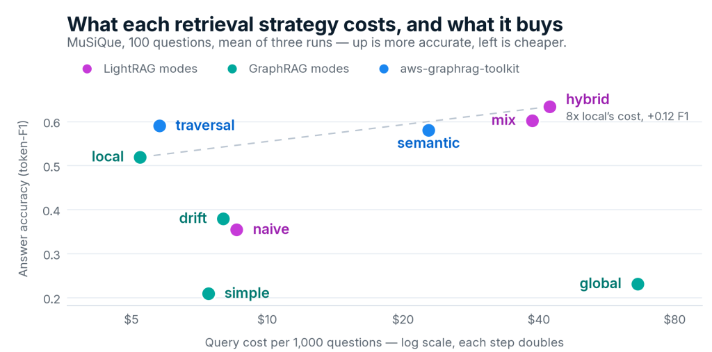
Answer accuracy against query cost per 1,000 questions — up is more accurate, left is cheaper. Cost is on a log scale, so each equal step to the right doubles the price and the 8x gap between local and hybrid is a constant width. Green squares are aws-graphrag-toolkit, included because it solves the same problem on the same AWS services. Exact figures are in the table above; every point is the mean of three runs, so read differences under about 0.05 as noise.
That cost column covers query cost only, and the two methodologies spend at different points: GraphRAG summarizes every community before the first question arrives, while LightRAG skips that step. The hidden cost is smaller than expected, though — on one corpus, community summarization was 7.6% of the total ingestion bill, because the dominant cost is extracting entities and relationships from every document, which both methodologies need.
The headline trade-off is that the most accurate strategy costs eight times the cheapest graph strategy: hybrid gains about 0.12 F1 over local at eight times the cost and three times the latency. Whether that matters is entirely a question of volume — at 1,000 questions a month it is $42 against $5, and at 100,000 it is $4,229 against $523, where the same 0.12 F1 now costs $3,700 a month. Four rules of thumb follow:
- Accuracy first, volume modest → hybrid or mix, if a 20-second response is acceptable and an 8x cost multiplier is affordable. In the low thousands of questions per month, it usually is.
- Volume past that, or answers needed in under 10 seconds → local, at roughly 82% of hybrid’s accuracy for an eighth of the cost.
- Single-fact lookups rather than multi-hop → evaluate plain vector search before adopting a graph at all. A graph earns its cost on the questions that need hops.
- Inspecting what the graph knows about one entity → simple, but not as a general-purpose answering strategy. It sits last in the table for a reason worth knowing: it queries every index at once and keeps the ten highest-scoring items, and since short questions match short text, descriptions crowd out the passages that hold the answer. It declines on 56 of 100 questions where naive — same slot count, passages only — declines 34.
If that lands you on the LightRAG side, you can also drop the indexing cost by setting graph.community_detection.enabled: false. Community detection is optional by design: global and drift need it, the LightRAG modes do not.
Where it falls short
global is not the strategy for thematic questions — even though thematic questions are what it is for. Community summaries cover the whole corpus, so they ought to answer “what are the themes here?” Testing that needed genuinely thematic questions, which neither benchmark above provides, so the test used 28 from UltraDomain with an LLM judge comparing answers head-to-head. global answers them without refusing, in well-structured syntheses — but wins only 64% against plain vector search, which at this sample size is not distinguishable from chance. mix wins 93% and local 82%.
The reason is variety, not volume. global assembled 4.2 context items per question against mix’s 134.8, yet the totals are closer than that ratio suggests — so it isn’t short of material. Four long summaries describe the corpus at one level of abstraction; 135 shorter items reach into many different documents, which gives the answering model more distinct things to reason from.
Cost compounds the problem. At $66.22 per 1,000 questions global is the most expensive strategy measured, because answering one question takes about 17.6 LLM calls as the map-reduce reads batches of summaries and combines partial answers. That also makes it the only strategy whose per-query cost scales with corpus size rather than with how much it retrieves — more documents means more communities to read on every question, so growth makes each question dearer instead of spreading the cost. Use global when a corpus-wide narrative is itself the deliverable; use mix when you want the best answer — including for questions that sound thematic.
Compared against the other AWS option
AWS already ships another project doing graph RAG on Neptune and OpenSearch: aws-graphrag-toolkit’s lexical-graph, which does not set out to reproduce either paper and instead builds its own graph of topics, statements, and facts. Its stronger mode differs by dataset, so each row below faces the better one:
| dataset | strongest here | strongest toolkit mode | difference | 95% CI |
|---|---|---|---|---|
| MuSiQue | hybrid 0.634 | traversal 0.590 | +0.04 | −0.00 to +0.09 |
| 2Wiki | mix 0.654 | semantic-guided 0.652 | +0.00 | −0.05 to +0.05 |
There is no accuracy advantage to claim in either direction. Both comparisons ran three replicates per side; significance is computed on the 300 pooled per-question scores, not on the three run means, and both intervals contain zero. Two independently built implementations landing on the same score suggests the benchmark is measuring the task rather than either codebase.
At the cheap end the ranking is clearer, and it does not favor this framework. For essentially the same money — $5.77 against $5.23 per 1,000 questions — the toolkit’s traversal mode scores 0.590 against local’s 0.519 and returns slightly faster, a gap large enough to be significant (95% CI −0.12 to −0.02). If query cost is the binding constraint, that is the arm to look at first.
Two conditions apply to every row. Both projects decline a comparable share of questions (11–20% and 11–19%, scored as zero either way), so neither gains from that convention. And each was left on its own default embedding model rather than forced to match, since defaults are what you would deploy — then the choice was measured, and it moves retrieval by less than run-to-run noise on these corpora.
So accuracy is not the basis for choosing between them. Reach for the toolkit when per-query cost is the binding constraint; reach for this framework when you need the retrieval behavior a paper describes, or when you want to compare strategies against each other on your own corpus.
How far to trust these numbers
- Every conclusion is scoped to these two benchmarks. Two datasets were enough to reverse the top two strategies and move individual scores by 0.16 F1; a third would likely reshuffle again.
- 100 questions detects a difference of about 0.1 F1 but cannot prove two strategies equivalent — that needs thousands. Read “matching” as “no difference we can detect”.
- Treat any single-run difference under about 0.05 as noise, and expect that band to depend on the strategy. Variation ranged from 0.000 to 0.025, and the zero is not a rounding artifact: naive and simple returned identical answers across three runs, because generation is greedy and neither asks an LLM to decide what to retrieve. The ones that do — mix, hybrid, and local extract keywords or entities first — are the ones that move.
- One graph per corpus, one judge family. Extraction is an LLM step, so these numbers rest on one particular graph; and on the thematic benchmark the judge shares a model family with the generator, a self-preference risk that applies to every strategy equally.
autowas not benchmarked. It routes between strategies; the numbers above are for the strategies it routes to.
Everything above ran on public corpora with public benchmarks. run-eval writes out the per-query answers and retrieved contexts that every figure here was computed from — token-F1 and the win rates were scored from those files afterwards, rather than by run-eval itself, so reproducing a number means re-running the arm and re-scoring its output. More usefully, you can point the framework at your own documents and find out which of these conclusions survive there.
Clean up
If you deployed the optional AWS CDK application, remove its resources when you no longer need them to avoid continuing charges for Amazon Neptune, Amazon OpenSearch Service, and, in public network mode, NAT gateways:
cd iac && cdk destroy --allThe default dev profile sets removal_destroy=true, so this deletes the stack’s stateful resources. Production configurations can retain resources or enable deletion protection. Review the CloudFormation stacks and iac/README.md, and remove any retained resources deliberately.
Wrapping up
Our compliance analyst’s question — which obligations are exposed if one milestone slips — is the kind that a knowledge graph is shaped to answer and a vector index is not. Unified Knowledge Graph RAG on AWS puts that capability on managed AWS services, with triple-hybrid retrieval and incremental indexing on a hexagonal, registry-driven stack, and it gives you two proven methodologies over one shared graph, switchable a query at a time.
Which one to reach for is a question the benchmarks answer better than intuition does. The short version: mix and hybrid give the strongest answers, local gives about 82% of that accuracy for an eighth of the cost, and global is for a corpus-wide narrative rather than the sharpest answer. When you are unsure, auto will route for you. And because both methodologies run over the same ingested graph, trying the other one is a configuration change rather than a re-index — which makes the cheapest useful experiment asking the same question two ways and comparing.
That experiment is worth running on your own corpus, because the one conclusion we would stand behind everywhere is that these rankings move when the questions change. Point it at your documents, turn on the DynamoDB registry so re-runs stay incremental, and — if your domain is specialized — run run-prompt-tuning first to adapt the extraction prompts. If you want to extend it rather than just use it, the registry-driven design means a new retrieval strategy or storage backend is an additive change, not a fork. Issues and pull requests are welcome.
- Repo: https://github.com/awslabs/unified-kg-rag-on-aws (Apache-2.0) — see CONTRIBUTING.md
- Upstream methodologies (companion reading): Microsoft GraphRAG (arXiv:2404.16130) and LightRAG (arXiv:2410.05779)