AWS Quantum Technologies Blog
Exact simulation of Quantum Enhanced Signature Kernels for financial data streams prediction using Amazon Braket
This post was contributed by Ernesto Palidda and Marco Paini from Rigetti Computing, Cristopher Salvi and Antoine Jacquier from Imperial College London, Samuel Crew from National Tsing Hua University and Shaun Geaney from Standard Chartered along with Sebastian Stern and Michael Brett from Amazon Web Services (AWS).
Empirical evidence suggests that well-chosen quantum feature maps promise to enhance the performance of Machine Learning (ML) algorithms. In this work, we harness the capabilities of the Amazon Braket SV1 on-demand state-vector simulator to experimentally test the use of quantum enhanced signature kernels up to 32 qubits to predict the mid-price using Limit Order Book (LOB) data.
Background
Imperial College London, Rigetti Computing, and Standard Chartered were awarded an Innovate UK grant to develop Quantum Machine Learning (QML) techniques for financial data streams. Standard Chartered provided a challenging use case with complex market microstructure data for which strong classical benchmarks exist. The team at Imperial has developed a state-of-the-art algorithm to compute signature kernels [1] which provide an effective method to implement kernel-based learning using path signatures as feature maps. The application team at Rigetti has collected numerical evidence of the benefits of introducing quantum transformations with specific properties within classical ML pipelines. AWS has supported the work with access to quantum circuit simulation resources on Amazon Braket. The experiments and results reported in this blog have been conducted as part of the Innovate UK grant.
While the goal of this research is to be able to execute QML algorithms on quantum hardware, the level of noise in currently available NISQ devices affects the ability to get an accurate measure of their effectiveness. Therefore, it is important to be able to validate the potential of the method based on simulation without noise. On the other hand, the computational resources required for an exact simulation increase exponentially with the qubit count. In this context, access to the Amazon Braket SV1 simulator, allows us to perform exact simulations of up to 34 qubits.
Use case description
Market making and execution are sophisticated activities that require methods to efficiently capture the market microstructure dynamics. Due to the size of the tick and the development of High-Frequency Trading this is an increasingly complex problem. Being able to predict the mid-price movements in the future allows adequate positioning.
The raw data available in the market is called Limit Order Book (LOB). Microstructure data consists of a list of pairs, volume and price, together with the direction, buy or sell. The number of pairs retained determines the depth of the LOB dataset. In equity markets the snapshots of the LOB are provided with a very high frequency. Therefore, LOB datasets are high-dimensional and very large. LOB data is proprietary, and its access is either restricted or expensive. The FI-2010 dataset has been made publicly available [2] and consists of 10 days of LOB data for 5 stocks on the NASDAQ OMX Nordic at the Helsinki stock exchange. Since then, it has been used as a benchmark dataset to test market microstructure models and trading strategies [3]. Additionally, the dataset is used to evaluate the DeepLOB model [4], which is a strong classical benchmark for this use case.
We use the FI-2010 LOB data to predict the mid-price movements 10 ticks ahead. For each of the 5 stocks the LOB data consists of 40 features. The mid-price prediction problem is modeled as a multi-class classification problem with 3 possible labels corresponding to the movements of the mid-price (upwards, downwards or stationary), where stationary is defined as the absolute price change being lower than 0.2 basis points. The benchmark models are trained on around 200,000 points and tested on around 60,000 points. We believe QML algorithms show a better approximation-generalization tradeoff than classical methods and are likely to show a separation against classical ML algorithms when training on a few data points. This was empirically observed on discrete logarithm type problems. In our quantum experiments, we use a sample of 1,000 consecutive training points and 1,000 consecutive testing points. The scale of our problem was determined by the number of training and testing points, the depth of the circuit, and the observables we want to measure; therefore, we reduced the number of features in our experiments from 40 features in the raw dataset to 12, 16, 24, and 32 features. We find that this dimension reduction has only a small impact on the performance of the model. To reduce the dimension of the input data, we truncate the number of features of the LOB dataset. When presenting a result using n features, it means that we have truncated the data at n/2 pairs.
Algorithm description
Signature Kernel: effective kernel trick for signature feature maps
Rough path theory has played a key role in the design of state-of-the-art machine learning algorithms for processing irregularly sampled, noisy and high-dimensional data streams. The signature of a path, a centerpiece of the theory, provides a top-down description of a signal by capturing its essential information, such as the order of events occurring, and filtering out potentially superfluous information like the sampling rate of the signal. The exponential explosion of signature features makes their application to high-dimensional streams difficult. Nonetheless, inner products of signatures provide a “dual”, seemingly more amenable, learning approach. The efficient and fast computation of these objects — through well-designed kernel tricks based on recent works [1] led by Imperial College London unveils a surprising connection between signatures and a class of hyperbolic partial differential equations allowing one to benefit from the advantages of working with infinitely many signature features without some of the concomitant drawbacks.
Quantum Feature Maps and Quantum Enhanced Signatures
Empirical evidence suggests that applying a feature map to the raw data prior to computing the path signature improves the performance of the downstream ML model to which the signature is passed. Typical classical feature maps that are used in the literature are Random Fourier Features or monomials of the original features. The Rigetti team has collected evidence to suggest that specific quantum feature maps outperform classical feature maps. For example, we demonstrated how combining a quantum feature map with a signature kernel can improve the predictions of recession in the US economy [5]. In other experiments the team has focused on using quantum feature maps in combination with an outlier detection method based on Chebyshev’s inequality. Initial results have been presented in the workshop Quantum Algorithms for Financial Applications at IEEE Quantum Week 2024. More importantly, theoretical arguments suggest the specific property that makes these quantum transformations useful for ML purposes is the amount of ‘magic’ of the output state of a circuit defining the quantum feature map.
The quantum feature map used in this work is constructed as follows. We start from an n-qubit state where n is the number of input features and the initial state will be the ground state |0>. We apply a ‘high-magic’ unitary transformation, namely one that produces an output state with a high stabilizer norm. We refer to [6] for a definition of the stabilizer norm and its link to magic of quantum states. This transformation is defined by a circuit where we repeat a fixed block composed of layers of single and two-qubit gates followed by an ‘encoding’ layer composed of single-qubit Z rotation gates with the rotation angle being determined by the value of the feature after scaling. The resulting quantum circuit is shown in Figure 1. The scaling used to ‘load’ the classical data in the circuit is called the bandwidth of the quantum feature map[a]. We compute the expectation values of Pauli observables (X, Y, Z) for every qubit and use these as quantum features. We therefore map n classic features into 3 * n quantum features. This feature map is equivalent to the projected quantum kernel algorithm [7]. We transform the original LOB data using this quantum feature map and apply the signature kernel on the transformed data.
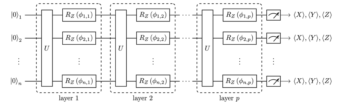
Figure 1: Circuit diagram of the quantum feature map for an n-qubit state consisting of p layers of a unitary transformation followed by single-qubit Z rotations with angles defined by the scaled values of the classical features. For every qubit, the expectation values of the Pauli observables X, Y, and Z are computed to map the n classical features into 3*n quantum features.
It is important to note that in the current implementation of our quantum enhanced signature kernel algorithm, the unitary transformation that defines the quantum feature map is fixed, its parameters are not trained. We perform a global search of the two hyperparameters that define the circuit associated with the unitary transformation: namely the bandwidth and the depth of the circuit i.e. the number of repetitions of the blocks. Therefore, our method is not adding trainable parameters and avoids the shortcomings associated with training parametric quantum circuits seen in reference [8].
The signature kernel pipeline is trained using a classical cross-validation approach. We train on around 885 points and test on 115 points. We then shuffle the training and testing points and choose the best set of parameters. The only free parameter of the model is the regularization term of the SVC classification model. Note that the dimension of the feature map does not impact the number of classically trainable parameters of the model. By using the kernel trick, the number of parameters that are classically trained by cross-validation is equal to the number of training points. This ensures that our quantum-classical comparison is fair, as we are not adding any trainable parameter to the model except the bandwidth and depth of the circuit, which are not trained. Additionally, the Quantum Enhanced Signature Kernel (QSK) model trained on 1,000 or even 5,000 points has fewer trainable parameters than the Deep LOB model which has around 60,000 trainable parameters.
Numerical Results
| Classical/Quantum | Model | Accuracy | Precision | Recall | F1 | Weighted Precision | Weighted Recall | Weighted F1 |
|---|---|---|---|---|---|---|---|---|
| Classical | Signature kernel, q=32 | 48.79% | 34.67% | 36.68% | 33.81% | 48.79% | 48.79% | 46.25% |
| Classical | Adaboost, q=16, on 1000 points | 57.73% | 44.78% | 43.46% | 43.57% | 55.95% | 57.73% | 56.68% |
| Classical | DeepLOB, q=32 | 48.26% | 31.25% | 32.24% | 27.60% | 42.37% | 48.26% | 40.05% |
| Quantum | QSK, q=32, d=96 | 49.95% | 35.15% | 35.60% | 35.18% | 48.23% | 49.95% | 48.85% |
| Quantum | QSK, q=12, d=12 (Rigetti QVM) | 70.35% | 53.74% | 52.97% | 52.79% | 68.28% | 70.35% | 69.14% |
| Quantum | QSK, q=16, d=48 (Rigetti QVM) | 68.66% | 50.74% | 51.15% | 50.62% | 66.62% | 68.66% | 67.50% |
| Quantum | QSK, q=24, d=56 | 70.03% | 49.25% | 51.01% | 49.98% | 67.61% | 70.03% | 68.71% |
| Classical | DeepLOB, q=40, full data set | 73.50% | 73.64% | 73.45% | 73.47% | 73.77% | 73.48% | 73.55% |
| Classical | Adaboost, q=16, full data set | 62.99% | 63.52% | 63.13% | 62.97% | 63.68% | 62.99% | 62.98% |
Table 1: Comparison of Quantum Enhanced Signature Kernel (QSK) performance against classical benchmarks across different feature dimensions.
Table 1 shows the comparison between QSK models against classical benchmarks across different feature dimensions for the prediction of the mid-price movements of the LOB of one stock. The first column on the left indicates whether the ML model is classical or quantum. In the second column, the notation “q=n” indicates that we have used n features, corresponding to choosing a LOB of depth n/2, and that the circuit uses n qubits. The notation “d=p” indicates that the depth of the circuit (defined as the repetition of the fixed block) is equal to p. “Full data set” indicates that the results correspond to the full original dataset, as for example the ones published in [4][b]. The weighted version of the metrics, given in the last three columns, are obtained assuming that the three classes of the problem are balanced. The original problem is unbalanced and the number of points corresponding to the stationary class is significantly smaller than the number of points in the other classes. For reduced samples of the original LOB problem we find a bandwidth and depth such that quantum enhanced signature kernels outperform classical signatures and other benchmark models by a significant margin. Moreover, the performance of quantum enhanced signatures obtained when training on 1,000 data points is comparable with the performance of the benchmark model trained on the full dataset of 200,000 points. These results seem to indicate that QML models are suitable for problems of this type with a small number of training points[c].
Finding the optimal circuit remains a difficult task as the search is costly as the qubit count grows. This appears clearly when comparing the results obtained at 32 qubits with lower qubit count. As detailed in the following section, the execution time of the 32 qubits runs did not allow us to run enough experiments to optimize the model hyperparameters. However, we have been able to identify some recurring patterns that helped us choose the hyperparameters.
| QSK, q=12, d=12 (Rigetti QVM) | |||||||||
|---|---|---|---|---|---|---|---|---|---|
| # test points | # train points | Batch # | Accuracy | Precision | Recall | F1 | Weighted Precision | Weighted Recall | Weighted F1 |
| 1000 | 1000 | 1 | 70.35% | 53.74% | 52.97% | 52.79% | 68.28% | 70.35% | 69.14% |
| 1000 | 1000 | 2 | 68.77% | 47.05% | 48.45% | 46.86% | 64.61% | 68.77% | 65.44% |
| 1000 | 1000 | 3 | 66.77% | 44.61% | 48.51% | 46.23% | 62.51% | 66.77% | 64.23% |
| 1000 | 1000 | 4 | 61.41% | 43.12% | 44.28% | 43.49% | 58.56% | 61.41% | 59.86% |
| 3000 | 5000 | 1 | 61.50% | 40.87% | 45.09% | 42.70% | 56.80% | 61.50% | 58.83% |
| 3000 | 5000 | 2 | 67.47% | 44.56% | 49.10% | 46.72% | 61.39% | 67.47% | 64.28% |
| 3000 | 5000 | 3 | 66.72% | 44.28% | 48.97% | 46.37% | 61.34% | 66.72% | 63.73% |
| 3000 | 5000 | 4 | 51.10% | 48.70% | 49.31% | 45.46% | 62.04% | 51.10% | 54.88% |
Table 2: Stability of the 12-qubit optimal circuit across different batches of data.
Table 2 compares the performance of the QSK across different batches of data for the prediction of the mid-price movements of the LOB of one stock. All the results are obtained using 12 features and a quantum feature map generated by a circuit of 12 qubits and depth 12 with the same bandwidth. The depth and bandwidth of the circuit have been chosen based on the performance of QSK on the first batch of data points. We observe that “optimal” circuit performance is robust across different batches of data (distant batches, which can be identified by the difference in the batches indices, perform less well suggesting different regimes). The optimal circuit determined on a single batch of points also performs when training on a larger set of points.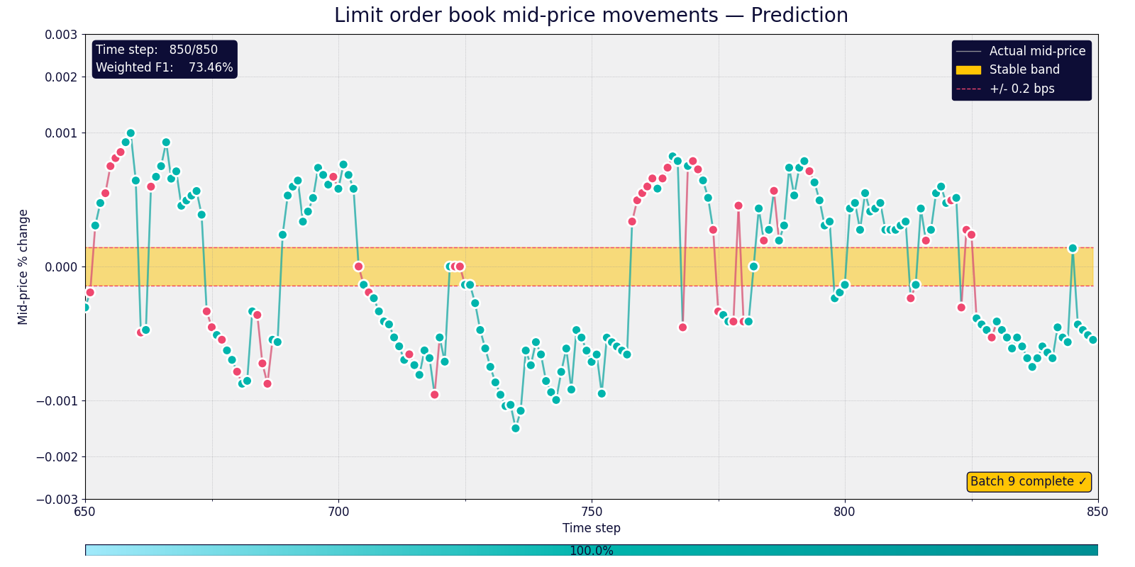
Figure 2: Step by step prediction of the mid-price movements of the LOB using the Amazon Braket SV1 on-demand simulator.
In Figure 2 each dot corresponds to a point of the test dataset. The yellow band in the middle of the figure indicates the area where the label is set to 1 (stable), the two grey areas correspond to the areas where the labels are 0 (price moving up) and 2 (price moving down). The dots and lines between dots are colored in red if the prediction of the quantum model is incorrect, or green if the prediction of the quantum model is correct. The figure is a snapshot of an animated graph which was presented at the AWS Summit London in April 2025. The snapshot shows the last 200 steps of 850. The Weighted F1 metric on the top left of the figure is computed on the full 850 points data set.
Workload dimensions and execution
The results discussed above were obtained with the SV1 on-demand simulator on Amazon Braket. SV1 is fully managed by AWS meaning there is no need to provision the underlying compute infrastructure or install any software. SV1 can perform full state vector simulation on demand for circuits with up to 34 qubits with or without shot noise and offers concurrent execution of up to 100 circuits.
We implemented the quantum circuit introduced in the algorithm description section using the programming constructs of the Amazon Braket Python SDK and ran several experiments with up to 32 qubits. The quantum model performance has been tested on batches of 1,000 training points and 1,000 testing points. To evaluate the performance of one circuit instance given a choice of depth and bandwidth we run 2,000 simulation tasks. Using the full concurrency of SV1 we split our batch of 2,000 tasks into 20 chunks of 100 tasks running in parallel on Braket.
In every task we compute 3 * n expectation values of local Pauli observables[d], for example: 96 observables for a 32-qubit circuit. As we were interested to validate the potential of our quantum feature map under ideal conditions, we ran exact simulations without shot noise and leveraged the fact that in that case we can simultaneously measure non-commuting observables like <X>, <Y>, and <Z> at once as previously mentioned in another post. On a real QPU we would not be able to measure non-commuting observables, meaning for one data point we would have to execute up to 96 circuits.
In summary, for the validation of our quantum feature map we ran about 7,000 quantum tasks at 32 qubits and 32,000 quantum tasks at a lower qubit count. Lower qubit runs between 20 to 28 qubits were used to both test the functionalities of the SV1 simulator and in the attempt to find a relationship between the number of qubits and the optimal depth of the circuit. We were able to complete the 7,000 32-qubit tasks within 156 hours. On average one task took 133 minutes and 30 seconds to run. The 28 qubits tasks took on average 311 seconds to run, while the 24 qubits tasks took on average 5 seconds to run.
Conclusion
Using Amazon Braket SV1 on-demand simulator we have experimentally tested the use of quantum enhanced signature kernels up to 32 qubits to predict the mid-price using LOB data. We have compared the performance against state-of-the-art classical benchmarks. We find that on small batches of data the quantum model outperforms classical benchmarks. We find that the performance of the quantum model trained on a small batch of data is close to the performance of the state-of-the-art classical benchmark trained on the full dataset. Also, the performance of an ‘optimally’ selected quantum model on one batch of data performs similarly on other batches of data, suggesting some stability/robustness of the optimal quantum model.
Implementation of such models on quantum hardware still presents several challenges. Among these, the most important is probably the fact that the proposed method suffers from a form of ‘exponential concentration’. For example, at 32 qubits, with circuit depth 96, the quantum features are of the order of magnitude of 10^(-5) or smaller. Even in the absence of hardware noise, this would require at least 10 billion shots to be able to obtain an accurate estimate of such quantities. The Rigetti team is currently investigating methods to mitigate such behavior of the model. We are considering using a different set of observables which tend to concentrate less than Pauli observables and limit the depth of the circuit to a logarithmic depth in the number of qubits.
In August 2025, the team at Imperial released a preprint introducing a novel signature-based framework adapted to quantum processes [9]. This work extends the classical theory of path signatures into the quantum domain, enabling a systematic way to encode and compare quantum trajectories. The formalism developed therein complements the methods presented in this blog post, and we anticipate that combining both classical and quantum signature representations will unlock new avenues for hybrid algorithm design and analysis.
Footnotes
[a] We rescale the values of the features using a min-max scaler, where the center of the interval is π/2 and the width is 2 times the bandwidth parameter. For example, if the center is π/2 and the bandwidth parameter is also equal to π/2, then the values of the features will be scaled between 0 and π.
[b] This GitHub repository referenced in the paper reproduces the results of [4], independently. The level of accuracy obtained differs slightly from the accuracy of the original paper, because we have reduced the size of the time window used in the model. The original paper uses a deep convolutional neural network where the convolution is made on 100 data points. By analogy, we could use a signature of a window of 100 data points. However, to keep the execution times down, we have reduced the size of the window to 50 data points.
[c] This has also been observed on artificial datasets such as a discrete logarithm type dataset. The results of these experiments were part of the presentation of the Rigetti team at IEEE Quantum Week 2024.
[d] In some of the simulation runs, we have computed 3 * n + 9 * (n-1) expectation values of local Pauli observables, 3*n single-qubit and 9*(n-1) two-qubit Pauli observables for all the neighboring qubits in the lattice. We assume that the lattice topology is a linear chain.
References
|
[1] |
C. Salvi, T. Cass, J. Foster, T. Lyons and W. Yang, “The Signature Kernel is the Solution of a Goursat PDE,” Siam Journal on Mathematics of Data Science, vol. 3, no. 3, pp. 873-899, 2021. [Online]. Available: https://arxiv.org/abs/2006.14794. |
|
[2] |
A. Ntakaris, M. Magris, J. Kanniainen, M. Gabbouj and A. Iosifidis, “Benchmark dataset for mid‐price forecasting of limit order book data with machine learning methods,” Journal of Forecasting, vol. 37, no. 8, pp. 852-866, 2018. [Online]. Available: https://arxiv.org/abs/1705.03233. |
|
[3] |
A. Briola, S. Bartolucci and T. Aste, “Deep limit order book forecasting: a microstructual guide,” Quantitative Finance, vol. 25, no. 7, pp. 1101-1131, 2025. [Online]. Available: https://arxiv.org/abs/2403.09267. |
|
[4] |
Z. Zhang, S. Zohren and S. Roberts, “DeepLOB: Deep Convolutional Neural Networsk for Limit Order Books,” IEEE Transactions on Signal Processing, vol. 67, no. 11, pp. 3001-3012, 2019. [Online]. Available: https://arxiv.org/abs/1808.03668. |
|
[5] |
M. Paini, E. Palidda, D. Garvin, C. Salvi, R. Malamud, A. Boughton, S. Gago, R. Garcia, E. Gaus and A. Jacquier, “Recession Prediction via Signature Kernels Enhanced with Quantum Features,” Moody’s Analytics Blog Post, 2023. [Online]. Available: https://www.moodys.com/web/en/us/about/what-we-do/quantum-computing/recession-prediction.html. |
|
[6] |
M. Howard and E. Campbell, “Application of a Resource Theory for Magic States to Fault-Tolerant Quantum Computing,” Physical Review Letters, vol. 118, no. 9, 2017. [Online]. Available: https://arxiv.org/abs/1609.07488. |
|
[7] |
H. Huang, M. Broughton, M. Mohensi, R. Babbush, S. Boixo, H. Neven and J. McClean, “Power of data in quantum machine learning,” Nature Communications, vol. 12, no. 1, 2021. [Online]. Available: https://arxiv.org/abs/2011.01938. |
|
[8] |
J. McClean, S. Boixo, V. Smelyanskiy, R. Babbush and H. Neven, “Barren plateaus in quantum neural network training landscapes,” Nature Communications, vol. 9, no. 1, 2018. [Online]. Available: https://arxiv.org/abs/1803.11173. |
|
[9] |
S. Crew, C. Salvi, W. Turner, T. Cass and A. Jacquier, Quantum Path Signatures, arXiv:2508.05103 [quant-ph], 2025. [Online] Available: https://arxiv.org/abs/2508.05103. |