AWS Quantum Technologies Blog
Simulating quantum circuits with Amazon Braket
Whether you want to research quantum algorithms, study the effects of noise in today’s quantum computers, or just prototype and debug your code, the ability to run large numbers of quantum circuits fast and cost effectively is critical to accelerate innovation. This post discusses the different types of quantum circuit simulators offered by Amazon Braket and its SDK. We look at the characteristics of each simulator, their differences, and when or why to use each one.
Today’s quantum computers still have limited capacity, qubit counts, and accuracy. Therefore, quantum circuit simulators, which emulate the behavior of quantum computers using classical hardware, are often the tool of choice to study quantum algorithms for quantum computing researchers and enthusiasts. Amazon Braket provides a suite of quantum simulators for different use cases to help customers prototype and develop quantum algorithms.
Overview of Amazon Braket simulators
The most common use case for simulators is to prototype, validate, and debug quantum programs. Whether you want to understand the foundation of Simon’s algorithm, or validate that your variational algorithm runs without a bug before running it on a quantum computer, it is useful to have a quick way to run small-scale circuits. For this reason, the Amazon Braket SDK comes pre-installed with a local simulator that runs wherever you use the SDK, for example, on Amazon Braket notebooks, or your own laptop.
Here is an example of how you can set up the local simulator in the Amazon Braket SDK and run a circuit:
# import libraries
from braket.circuits import Circuit, Gate, Observable
from braket.devices import LocalSimulator
from braket.aws import AwsDevice

# instantiate local simulator
device = LocalSimulator()

# define the circuit
bell = Circuit().h(0).cnot(0, 1)
# run the circuit
result = device.run(bell, shots=1000).result()

# print the results
print(result.measurement_counts)

[out]: Counter({'00': 517, '11': 483})
While the local simulator is great for small-scale prototyping and debugging, when you want to develop and research quantum algorithms you often need simulations at larger scale. To illustrate this point, let’s have a look at variational quantum algorithms, like the quantum approximate optimization algorithm (QAOA) or the variational quantum eigensolver (VQE), the workhorses of near-term quantum computing. In these algorithms, quantum circuits are parameterized and these parameters iteratively adjusted to find the solution to a problem, similar to the way machine learning models are trained.
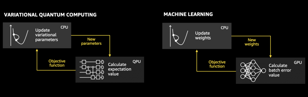
Figure 1. Variational quantum algorithms are based on the same principles as the training of machine learning models.
To understand the convergence and scaling behavior of these algorithms, researchers want to push their experiments to larger and larger qubit numbers. This has two implications. On the one hand, the simulation of each individual circuit, or task, becomes exponentially harder with the number of qubits (We’ll discuss exceptions to this in the TN1 section). On the other hand, larger problems generally require more circuit evaluations to calculate gradients and optimize the parameters of the circuits in your variational quantum algorithm. For instance, using the parameter shift rule, you need at least 50 circuit evaluations to calculate a single gradient for a circuit with 25 parameters.
To make the simultaneous computation of multiple complex circuits fast and performant, Amazon Braket provides three on-demand circuit simulators:
- SV1, a general-purpose state vector simulator
- TN1, a tensor network simulator for circuits with special structure
- DM1, a density matrix simulator for simulating circuits under the influence of noise
All three of these simulators provide customers with the scalability and performance of the AWS Cloud to compute batches of large circuits with minimal effort. You will need an AWS account to use the on-demand simulators, and you can use them either from your local developer environment or from a managed notebook instance.
To run a circuit, set your device to one of the on-demand simulators and run your experiments as usual:
# instantiate the SV1 device
device = AwsDevice("arn:aws:braket:::device/quantum-simulator/amazon/sv1")

# run circuit
result = device.run(bell, shots=1000).result()

print(result.measurement_counts)

[out]: Counter({'00': 504, '11': 496})
~
The results of your circuits are automatically computed on AWS managed compute infrastructure. There is no need for you to set up or manage hardware or simulation software. You only pay for what you use, that is, the time the simulation took to complete, with a minimum of three seconds. You don’t have to worry about idle infrastructure while you prepare your next experiment. To learn more about pricing, see the Amazon Braket pricing page or use our pricing calculator. Note, the use of Amazon Braket on-demand simulators is part of the AWS Free Tier, so you can use up to one hour of simulation time per month for your first year of usage.
Most importantly, all on-demand simulator devices can process many of your circuits in parallel, so you can scale large batches of tasks out to the cloud, speeding up the gradient computations when simulating variational algorithms. SV1 and DM1 can process up to 35 of your tasks in parallel, and TN1 up to 10. And running batches of tasks is easy: When using the Amazon Braket SDK, you can simply use the run_batch() function:
# a function to create an n-qubit “GHZ” state
def build_ghz_circuit(n_qubits):
    circuit = Circuit()
    # add Hadamard gate on first qubit
    circuit.h(0)

    # apply series of CNOT gates
    for ii in range(0, n_qubits-1):
        circuit.cnot(control=ii, target=ii+1)
    return circuit

# define a batch of GHZ circuits
ghz_circs = [build_ghz_circuit(nq) for nq in range(2, 22)]

# run the circuit batch
batch_tasks = device.run_batch(ghz_circs, shots=1000)

# print the first 3 task results

results = batch_tasks.results()

for result in results[:3]:
    print(result.measurement_counts)
[out]:
Counter({'11': 516, '00': 484})
Counter({'000': 510, '111': 490})
Counter({'1111': 501, '0000': 499})
Note that you are going to be billed for each simulation task individually, so if you run 10 tasks in parallel, you are accruing 10x the cost of an individual task.
If you use PennyLane, the Amazon Braket plugin makes sure that your gradients are computed efficiently if you set the parallel=True flag when instantiating the Amazon Braket simulator. In this tutorial, we show you how this parallel execution of circuits can significantly speed up gradient computations for variational algorithms.
SV1: Predictable performance scaled out in the cloud
So when should you use an on-demand simulator instead of the local one? To answer this question, look at SV1, our on-demand state vector simulator. State vector simulators are the workhorse of circuit simulation. They keep a precise representation of the quantum state (the state vector) at every point in the simulation, and iteratively change the state under the action of the different gates of the circuit, one by one. Each gate that is applied corresponds to a matrix-vector multiplication resulting in predictable runtimes of SV1 with little variation.
In a sense, state vector simulators have an advantage over QPUs: You cannot directly access the state of the quantum system within a QPU. You can only ever measure parts of it, and each shot, i.e., a single circuit execution and subsequent measurement, gives a small piece of information. The fact that you have to run a finite number of shots leads to small, probabilistic variations in the results, even if you had a perfect quantum computer without errors. These variations are generally referred to as shot noise, which decreases with the number of shots you run. Since state vector simulators have access to the full quantum state, you can sample measurement results, or shots, at negligible cost to better understand the effect of shot noise on your algorithm. This helps you select the right number of shots once you run on real quantum hardware. You can even choose to access the ideal results without shot noise to study your algorithm under ideal conditions by setting shots=0 like in the following example.
# define the circuit
bell = Circuit().h(0).cnot(0, 1)

# add a set of state amplitudes to the requested result types
bell.amplitude(state=["00","11"])

# run the circuit
result = device.run(bell, shots=0).result()

# print the results
print(result.values[0])

[out]:
{'00': (0.7071067811865475+0j), '11': (0.7071067811865475+0j)}
Moreover, on a QPU, you cannot simultaneously measure certain components of your system. For instance, if you want to measure the observables <X> and <Y> on a qubit, you need run two separate circuits that differ slightly. State vector simulators like SV1 do not have that limitation. You can request any number of observables, and SV1 only needs a single run to compute the results:
# define the circuit
bell = Circuit().h(0).cnot(0, 1)

# add non-commuting observables to the requested results
bell.expectation(Observable.Z(), target=[0])
bell.expectation(Observable.X(), target=[0])
bell.expectation(Observable.Y(), target=[0])
bell.expectation(Observable.X() @ Observable.X(), target=[0, 1])

# run the circuit
result = device.run(bell, shots=0).result()

# print the results
print(result.values[0])
print(result.values[1])
print(result.values[2])
print(result.values[3])

[out]:
0.0
0.0
0.0
0.9999999999999998
This can significantly speed up certain computations, in particular in the area of computational chemistry, where you often need to compute large sets of so-called non-commuting observables which, on a QPU, would require multiple tasks.
DM1: Study the effects of noise in quantum computers
State vector simulators like SV1 are a great way to explore the performance of quantum algorithms in the ideal case, in which no errors occur, and you can prepare and read out results perfectly. However, real quantum devices do experience a variety of errors, whether in applying gates, reading out results, or initializing the QPU. You can use DM1, the density matrix simulator, to explore the effects of noise on your circuits. This can help you understand how your algorithms might perform on a real-world quantum device, such as one of the QPUs available through Amazon Braket, and improve the reliability of your algorithms under real-world conditions. Similarly to SV1, DM1 must store a complete representation of the state of the system at each point in the simulation. Because the noise introduces classical uncertainty (Did a qubit accidentally flip or not?), this state, however, cannot be expressed as a single state vector, as in the noise-free case. Instead, the quantum state generally has to be expressed as a classical ensemble of different state vectors. This ensemble is called a density matrix, and it is the most general description of a quantum state, due to the additional degrees of freedom that need to be captured. As a rule of thumb, to store the density matrix of an N-qubit system, you need as much memory as you need to store a 2N state vector. Hence, DM1 supports circuits with up to 17 qubits instead of the 34 qubits that SV1 supports.
The Amazon Braket SDK provides a variety of ways to apply noise to your circuit. For example, you can introduce errors when initializing the qubits:
# import libraries
from braket.circuits import Circuit, Gate, Observable, Noise
from braket.aws import AwsDevice

# instantiate the DM1 device
device = AwsDevice("arn:aws:braket:::device/quantum-simulator/amazon/dm1")

# define the circuit
bell = Circuit().h(0).cnot(0, 1)

# add initialization noise to the circuit
bell.apply_initialization_noise(Noise.BitFlip(probability=0.1), target_qubits=1)
Or when reading out the results at the end of the simulation:
# add read out noise to the circuit

bell.apply_readout_noise(Noise.BitFlip(probability=0.1), target_qubits=0)
We can also apply noise to specific qubits, which affects every gate that touches those qubits, a specific gate type, for example targeting all H gates applied in the circuit:
circuit = Circuit()

n_qubits = 6
# add Hadamard gate on first qubit
circuit.h(0)

# apply series of CNOT gates
for ii in range(0, n_qubits-1):
    circuit.cnot(control=ii, target=ii+1)

# apply phase flip noise to all Hadamard gates
noise = Noise.PhaseFlip(probability=0.2)
circuit.apply_gate_noise(noise, target_gates=Gate.H)
Similar to SV1, DM1 provides both shots=0 and shots>0 measurements. For a full list of supported result types, you can look at the Amazon Braket Developer Guide. To learn more about the different ways of programming circuits with noise and running them on DM1 or the local simulator see the example notebook, “Simulating noise on Amazon Braket.”
You can also use noise simulation in PennyLane, for instance, to investigate the impact of noise on the convergence of variational algorithms. This notebook explains how to use noise simulation in PennyLane with the example of a QAOA algorithm.
TN1: Avoiding the memory explosion in simulating large circuits
Now, look at Amazon Braket’s tensor network simulator, TN1. TN1 works differently than SV1 and DM1, so it’s important to understand how TN1 simulates quantum circuits and how some circuits are easier to simulate with TN1 than others based on their structure. Note that TN1 is not available in the us-west-1 region.
As previously noted, state vector simulators keep track of the exact representation of the quantum state at every point during the simulation. That comes at great computational cost, as the required memory scales exponentially with the number of qubits. It turns out, however, you don’t actually always need the full state vector to get to the results you want. That’s where tensor network simulators come in: unlike a state vector simulator, a tensor network simulator doesn’t keep track of the amplitudes of all possible output states at every step in the circuit evaluation. Instead, a tensor network simulator like TN1 represents the gates of the circuit as vertices in a graph. The vertices are connected by edges which represent the incoming or outgoing qubits each gate is acting on. The following figure shows on the left the tensor network representation of a 34-qubit GHZ circuit, using the popular tensor network library Quimb, compared to the corresponding circuit representation on the right.
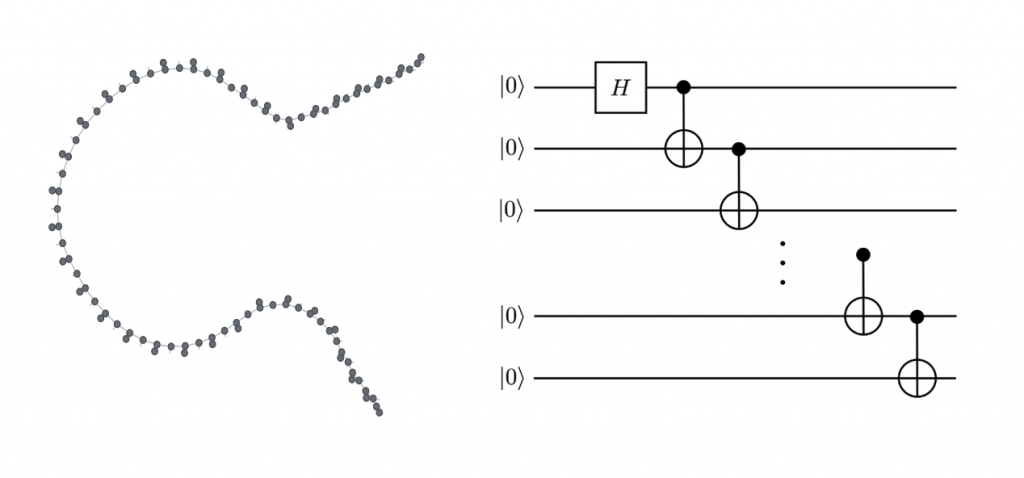
Figure 2. Tensor network representation of a GHZ circuit (left) and the corresponding circuit diagram (right)
The tensor network simulator then attempts to determine a good order in which to combine these nodes — any such order (or “contraction path”) will give the same end result, but the impact of order choice on performance can be substantial. Thus, the controlling factor that determines whether a circuit is easy to simulate with a tensor network simulator is not the number of qubits addressed in the circuit (as it is for SV1 or DM1), but rather how easy it is to find an order to combine the gates in a way that will allow the computation to be performed in a reasonable amount of time. In general, such a path exists and can be found quickly as long as the qubits of the circuit can be rearranged in such a way that the entanglement in the system throughout the computation is low and short range. Therefore, TN1 is best suited for circuits with local gates (i.e., gates acting only on neighboring or nearby qubits), low depth, or other structures that limit the spread of entanglement. To learn more about the kinds of circuits TN1 can best handle, you can follow the tutorial notebook “Testing the tensor network simulator with 2-local Hayden-Preskill circuits.”
To make this more concrete, let’s look at two examples. The first case is a so-called local Hayden-Preskill (HP) circuit. We will construct a random instance from this circuit class that preserves a local structure in the sense that only nearest neighbor qubits can have gates applied between them. Here is an example of a 4 qubit, local HP circuit with depth 12.

Figure 3. Circuit diagram of a 4 qubit, local Hayden-Preskill circuit with depth 12
For the second case, we will use another random circuit class, this time, where gate can be applied between all qubits without respecting any local structure. Here is an example of such a circuit with 4 qubits and depth 8.

Figure 4. Circuit diagram of an all-to-all connected circuit with 4 qubits and depth 8.
We will now investigate how TN1’s performance compares with SV1’s performance in each of these cases and draw some lessons about when each simulator is appropriate to use. Let us first consider a local HP circuit with 34 qubits, the maximal qubit count SV1 can simulate.
from braket.circuits import Circuit, Gate, Observable, Instruction
from braket.devices import LocalSimulator
from braket.aws import AwsDevice
import numpy as np
from math import pi

# prepare a local Hayden-Preskill circuit
def local_Hayden_Preskill(n_qubits, numgates, czrange=1):
    hp_circ = Circuit()
    """Yields the circuit elements for a scrambling unitary.
    Generates a circuit with numgates gates by laying down a
    random gate at each time step.  Gates are chosen from single
    qubit unitary rotations by a random angle, Hadamard, or a
    controlled-Z between a qubit and its nearest neighbor (i.e.,
    incremented by 1)."""
    qubits = range(n_qubits)
    for i in range(numgates):
        if np.random.random_sample() > 0.5:
            """CZ between a random qubit and another qubit separated at most by czrange."""
            gate_range = np.random.choice(range(1, czrange+1), 1, replace=True)[0]
            a = np.random.choice(range(n_qubits-gate_range), 1, replace=True)[0]
            hp_circ.cz(qubits[a],qubits[a+gate_range])
        else:
            """Random single qubit rotation."""
            angle = np.random.uniform(0, 2 * pi)
            qubit = np.random.choice(qubits,1,replace=True)[0]
            gate  = np.random.choice([Gate.Rx(angle), Gate.Ry(angle), Gate.Rz(angle), Gate.H()], 1, replace=True)[0]
            hp_circ.add_instruction(Instruction(gate, qubit))
    return hp_circ

lHP = local_Hayden_Preskill(34, 34*4)
sv1 = AwsDevice("arn:aws:braket:::device/quantum-simulator/amazon/sv1")
tn1 = AwsDevice("arn:aws:braket:::device/quantum-simulator/amazon/tn1")

tn1_task = tn1.run(lHP, shots=1000).result()
tn_runtime = tn1_task.additional_metadata.simulatorMetadata.executionDuration
print("TN1 runtime: ", tn_runtime)

sv1_task = sv1.run(lHP, shots=1000).result()
sv_runtime = sv1_task.additional_metadata.simulatorMetadata.executionDuration

print("SV1 runtime: ", sv_runtime)

[out]:
TN1 runtime:  18018
SV1 runtime:  815853
Comparing these runtimes, you see that for the local HP circuits, TN1 is almost two orders of magnitude faster than SV1.
On the other hand, TN1 is not always the best choice. Look at the second type of circuit noted previously, which features non-local or all-to-all connectivity:
# import libraries
from braket.circuits import Circuit, Gate, Observable, Instruction
from braket.devices import LocalSimulator
from braket.aws import AwsDevice
import numpy as np
import math

# a function to prepare an all-to-all circuit
def all_to_all(n_qubits, n_layers, seed=None):
    if seed is not None:
        np.random.seed(seed)
    def single_random_layers(n_qubits, depth):
        def gen_layer():
            for q in range(n_qubits):
                angle = np.random.uniform(0, 2 * math.pi)
                gate = np.random.choice([Gate.Rx(angle), Gate.Ry(angle), Gate.Rz(angle)], 1, replace=True)[0]
                yield (gate, q)
        for _ in range(depth):
            yield gen_layer()

	circ = Circuit()

    circs_single = single_random_layers(n_qubits, n_layers+1)

    for layer in range(n_layers):
        for sq_gates in next(circs_single):
            gate, target = sq_gates
            circ.add_instruction(Instruction(gate, target))

        # match the qubits into pairs
        x = np.arange(n_qubits)
        np.random.shuffle(x)
        for i in range(0, n_qubits - 1, 2):
            i, j = x[i], x[i + 1]
            circ.cnot(i, j)

    # last layer of single qubit rotations
    for sq_gates in next(circs_single):
        gate, target = sq_gates
        circ.add_instruction(Instruction(gate, target))

    return circ
The fact that there are many gates connecting qubits across the circuit allows entanglement to spread fast, making tensor network simulations difficult to perform. Or, in the mathematical language of tensor networks, the number of possible contraction orders is very high, and therefore it will be difficult for TN1 to find a good contraction path. Even if a path is found, it might be too hard to contract in reasonable time. Thus, you see that SV1 runs such a circuit much more quickly:
# define the circuit
circ = all_to_all(18, 10)

# instantiate the devices
sv1 = AwsDevice("arn:aws:braket:::device/quantum-simulator/amazon/sv1")
tn1 = AwsDevice("arn:aws:braket:::device/quantum-simulator/amazon/tn1")

# run the circuit on both devices
sv1_task = sv1.run(circ, shots=10).result()
tn1_task = tn1.run(circ, shots=10).result()

# print the runtime
sv_runtime = sv1_task.additional_metadata.simulatorMetadata.executionDuration
tn_runtime = tn1_task.additional_metadata.simulatorMetadata.executionDuration

print("SV1 runtime: ", sv_runtime)
print("TN1 runtime: ", tn_runtime)

[out]:
SV1 runtime:  27
TN1 runtime:  36006
Finally, in some cases, TN1 may not be able to find a single viable contraction order. In these cases, the task will not complete and end in the status FAILED:
circ = all_to_all(18, 30)
tn1_task = tn1.run(circ, shots=10).result()
[out]: Task is in terminal state FAILED and no result is available
You can query the failureReason to understand why your task didn’t succeed:
if tn1_task.state() == "FAILED":
    print(tn1_task._metadata['failureReason'])
As you can see, the number of qubits in your circuit is not the dominant factor controlling whether TN1 will be able to process it or not. Rather, the circuit’s geometry, depth, and generally its structure play a very important role. For circuits with local gates, limited depth, or other characteristics that may limit the build-up of entanglement in the circuit, TN1 can potentially provide significant speedups over SV1 and, in some cases, simulate circuits with qubit numbers that are out of reach for SV1 or other state vector simulators.
For more examples of the effect of circuit geometry on TN1, try working through the TN1 demo about the effects of gate locality.
Conclusion
Quantum circuit simulators are indispensable tools in quantum computing today, whether you are a researcher who is developing new algorithms or you are just getting started. In this post we introduced the different simulator devices available on Amazon Braket and demonstrated simple examples of how and when to use them. Amazon Braket simulators cover a variety of use cases, helping you to debug you code, test new algorithm ideas at scale, and understand the impacts of noise in real devices on the quality of your results. The following table summarizes the main use cases for each of the four Amazon Braket simulators.

Figure 5. Overview of the main use cases for the four Amazon Braket simulators
Additional simulators, developed by our partners or containerized in a Docker image, are also available through Amazon Braket Hybrid Jobs. These simulators, as well as the Local Simulator discussed in this post, can be run “embedded” within a job to keep all computations in the same environment. To learn more about embedded simulators, see the example notebook.
To learn more, you can read the Amazon Braket Developer Guide or follow the tutorials in the Amazon Braket example repo. These tutorials are also available on Amazon Braket notebooks to help you get started quickly.
Resources
Here are some example Jupyter notebooks in the Amazon Braket GitHub repo that can help you dive deeper into using simulators:
Getting started with Braket simulators