Optimization of robot trajectory planning with nature-inspired and hybrid quantum algorithms

Introduction

The problem of robot motion planning is pervasive across many industry verticals, including (for example) automotive, manufacturing, and logistics. In the automotive industry, robotic path optimization problems can be found across the value chain in body shops, paint shops, assembly, and logistics, among others [1]. Typically, hundreds of robots operate in a single plant in body and paint shops alone. Paradigmatic examples in modern vehicle manufacturing involve so-called welding jobs, application of adhesives, sealing panel overlaps, or applying paint to the car body. The common goal is to achieve efficient load balancing between the robots, with optimal sequencing of individual robotic tasks within the cycle time of the larger production line.

In this blog, we discuss our recent collaboration with the BMW Group to solve their robot motion planning problem. Our goal was to assess whether the robot motion planning problem could benefit from quantum computing. We specify the business problem definition, discuss multiple relevant problem formulations, introduce a set of solvers applied to the problem, and provide some results across the solvers, across multiple datasets. We leverage both classical (in particular, nature-inspired) and quantum computing-based approaches to solve the problem, and evaluate them directly against one another. To run the quantum solvers, we leverage tools available on Amazon Braket, including the QPU backends and notebook instances. We show how the overhead required to map the problem to a quantum annealer becomes prohibitive at industry-relevant scales, so while the quantum annealer performance is competitive on smaller instances, it cannot scale with the classical approaches. We show that the best solver, what we call the random key optimizer, consistently generates the best result across the full range of problem sizes, yielding a ~10% improvement over the greedy baseline for these same industry-relevant instances.

Problem definition

As part of its production line, BMW applies sealant with special compounds to welds on the car chassis to ensure water-tightness. Polyvinyl chloride (PVC) is commonly used, applied in a fluid state, thereby sealing the area where different metal parts overlap. The strips of PVC are referred to as seams. Post application, the PVC is cured in an oven to provide the required mechanical properties during the vehicle’s lifetime. Important vehicle characteristics such as corrosion protection and soundproofing are enhanced by this process.

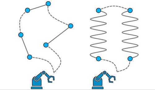
Figure 1. Schematic illustration of the use case. Robots are programmed to follow certain trajectories along which they apply a PVC sealant along seams. The seams are highlighted by solid lines with two endpoints each and are not necessarily straight. Dotted lines represent additional motion between seams. Every robot is equipped with multiple tools and tool configurations, to be chosen for every seam. The goal is to identify collision-free trajectories such that all seams get processed within the minimum time span.

Modern plants usually deploy a fleet of robots to apply the PVC sealant, as schematically depicted in Figure 1. However, the major part of robot programming is typically carried out by hand, either online or offline. Compared to the NP-hard traveling salesperson problem (TSP), the complexity of identifying optimal robot trajectories is amplified by three major factors: 1. an industrial robot arm can have multiple configurations that result in the same location and orientation of the end effector, 2. the PVC is applied with a tool that is equipped with multiple nozzles that allows for application at different angles, and 3. industrial robots are frequently mounted on a linear axis, thus an optimal location of the robot on the linear axis at which the seam is processed must be determined. The objective of selecting and sequencing the robot’s trajectories is to find a time-optimal and collision-free production plan such that all seams are processed exactly once. Such an optimal production plan may increase throughput, and automation of robot programming reduces the development time of new car bodies.

Problem formulations

At its core we can view the robot trajectory problem as a sequencing problem, wherein we must order the sequence to cover all elements in the sequence in minimal cost, where cost is total time to cover the tour of seams (while specifying all other degrees of freedom). This closely resembles the canonical TSP, and so we first discuss different potential TSP-style representations for the problem, and then generalize this approach to the real-world robot motion use case.

Native representation

The native representation is often the ideal formulation for any problem, yielding an efficient mathematical representation with a relatively small number of variables to be optimized. For the TSP, this means we hope to represent each element in the tour as an abstract node ID, and the time order of steps is implicit in the sequence of node IDs, which can be broken down so to calculate the cost of individual steps. Formally, a solution to the TSP is a permutation π of the n cities visited and its cost is

c=ℓ(π₁,π₂) + ℓ(π₂,π₃) + … + ℓ(π_n-1,π_n) + ℓ(π_n,π₁)

is the distance between city i and city j. Consider, for example, a TSP where we must cover four cities, which we label as the set {1, 2, 3, 4}. One potential solution π is simply the sequence [1, 2, 3, 4], and the cost for this solution would be

c=ℓ(1,2) + ℓ(2,3) + ℓ(3,4) + ℓ(4,1)

Notice we did not need to include any variable for time, and we were even able to implicitly represent the step from the final city to the home city by connecting the first and last elements of the sequence. Any constraints, for instance that the tour must be collision-free, can be included via a penalty in the form of a large cost for a step where that constraint is violated.

To extend this representation to our use case, we need to expand the node IDs to be a composite vector representing all relevant degrees of freedom (seam ID, tool ID, tool configuration, etc.). In our case, the node is a quintuple of the form

node = [s, d, t, c, p]

where a node encapsulates information about the seam index s=1, …, n_seams , the direction d=0,1 by which a given seam is sealed, the tool t=1, …, n_tools and tool configuration c=1, …, n_config used, as well as the (discretized) linear-axis position p=1, …, n_position. Thus, some example native sequence of nodes might look like

π = [[1,0,0,1,0],[2,1,1,0,0],[3,0,1,1,0],[4,1,1,0,0]]

It becomes the responsibility of the solver to ensure that the proposed tour covers all seams, which in the case of the biased random key genetic algorithm and the dual annealer is handled in an implicit manner. This will be covered in later sections.

QUBO representation

Current quantum hardware backends, especially annealers, require a QUBO (short for Quadratic Unconstrained Binary Optimization) formulation in order to be applied to a problem. The QUBO framework is a powerful approach that provides a common modelling framework for a rich variety of NP-hard combinatorial optimization problems [2, 3, 4, 5], albeit with the potential for a large variable overhead for some use cases. The cost function for a QUBO problem can be expressed in compact form with the Hamiltonian

x=(x₁, x₂, …) is a vector of binary decision variables and the QUBO matrix Q is a square matrix that encodes the actual problem to solve. Without loss of generality, the Q-matrix can be assumed to be symmetric or in upper triangular form [4]. We have omitted any irrelevant constant terms, as well as any linear terms, as these can always be absorbed into the Q-matrix because x_i²=x_i for binary variables x_i ∈ {0,1} .

For application to our problem, we introduce binary (one-hot encoded) variables, setting x^τ_node = 1 if we visit node=[s,d,t,c,p] at position τ = 1,…,n_seams of the tour, and x^τ_node = 0 otherwise.

If we take the toy solution sequence from the native formulation [3, 2, 4, 1], we would represent this solution as

x = [0,0,1,0, 0,1,0,0, 0,0,0,1, 1,0,0,0]

Note what was a sequence of length 4 now becomes length 16, as we must explicitly label each node as 0 or 1, and we must tile those binary node representations for each step. More generally, this binary encoding incurs a quadratic overhead consuming n² binary variables for a problem with n cities.

Extending this to our composite node representation (recall node = [s, d, t, c, p]) requires also encoding the additional degrees of freedom (direction, tool, configuration, and linear-axis dimensions).

Following the QUBO formulation for the TSP problem [2], we can then describe the goal of finding a minimal-time tour with the quadratic Hamiltonian

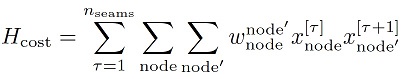
with w^node’_node denoting the cost to go from node to node’. Here, the product x^τ_nodex^τ+1_node=1 if and only if node is at position τ in the cycle and node’ is visited right after at position τ+1. In that case, we add the corresponding distance w^node’_node to our objective function, which we would like to minimize. Overall, we sum all costs of the distances between successive nodes.

At this point, we have no restrictions on the decision vector x^τ_node meaning we could (and likely would) yield infeasible solutions. To help drive the solver towards feasible solutions, we need to add penalty terms to account for the following constraints: 1. we must visit exactly one node per time step, and 2. all seams (not nodes) must be visited exactly once throughout the tour. Mathematically we can account for these constraints by adding additional penalty terms to our Hamiltonian:

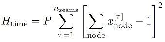
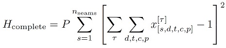
with the penalty parameter P>0 enforcing the constraints. Note that the numerical value for P can be optimized in an outer loop. Combining these penalty terms with our previous cost, the total QUBO Hamiltonian describing the use case then reads

Now that we have our relevant problem representations, we can discuss what tools and algorithms we’ll use to solve the problem.

Overview of solution strategies – from random keys to quantum annealing

Random Key Optimizer (RKO)

Our classical solutions are based on what we call the “random key optimizer” (RKO) framework. The RKO framework is based on the idea that a solution to an optimization problem can be encoded as a vector of random keys, i.e., a vector X in which each entry is a real number, generated at random in the interval (0,1]. Such a vector X is mapped to a feasible solution of the optimization problem with the help of a decoder, a deterministic algorithm that takes as input a vector of random keys and returns a potential solution to the optimization problem, as well as the cost of the solution, as shown in Figure 2. A search algorithm (see following) is responsible for generating these vectors X in an intelligent way, using the cost feedback from the decoder to improve the quality of generated vectors.

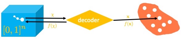
Figure 2. Schematic depiction of the RKO framework. The (blue) box on the left represents the abstract search space hosting all possible random-key vectors. The underlying optimization algorithm, for instance Dual Annealing (DA), will search this space, generating candidate random key vectors X as it searches. These random key vectors are passed to the decoder (yellow) to be converted into a corresponding cost (or fitness) f(X), by mapping the random-key vector into a solution x of the original problem; the cost f(X) is passed back to the search algorithm as feedback signal. The searcher uses the cost information to inform its next search step(s). When finished, the decoder can provide the final solution vector x and associated cost f(x) back to the parent process to be used downstream.

To see how this works, consider the TSP described previously with four cities. A possible decoder for the TSP takes the vector of random keys as input and sorts the vector in increasing order of its keys. The indices of the sorted vector make up π, the permutation of the visited cities. Now imagine the search algorithm proposes the random key X = (0.45, 0.78, 0.15, 0.33) – the sorted vector is s(X) = (0.15, 0.33, 0.45, 0.78) and its vector of indices is π = (3, 4, 1, 2), having cost

c=ℓ(3,4) + ℓ(4,1) + ℓ(1,2) + ℓ(2,3)

This is sufficient for the uni-dimensional case, but our use case is described by composite nodes that encapsulate multiple degrees of freedom. To handle this, we have to extend the decoder described previously to assign discrete values for the remaining node dimensions (beyond seam ID), as illustrated in the red block in Figure 3. For example, if the corresponding original variable is binary, as is the case in Figure 3, the thresholding logic reduces to int(X) ∈ {0,1} but generalizations to variables with larger cardinality are straightforward. For example, if a larger cardinality is assumed for the original variable Y_i, say Y_i ∈ {1,2,…,C}, then

Y_i=k if X_i ∈ ( (k-1)/C, k/C ] for k=1,2,…

In other words, if the dimension has C unique values, then we split the continuous range [0, 1] into C equal width bins and map the random key X_i to the appropriate bin label.

Note that our mathematical representation by design generates feasible routes only where every seam is visited exactly once, while only scaling linearly with the number of seams ~n_seams, and with a prefactor set by the number of degrees of freedom.

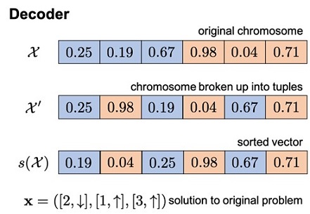
Figure 3. Example decoder logic. The search algorithm provides a random key vector X to the decoder to be decoded. Here, the vector of random keys X is made of two subunits (blue and red colored): one set of values to represent the seam ID (blue) and another set to represent the second dimension (red), which in this case is chosen to be binary (such as, for example, the direction variable). The elements of each subunit are then paired together, such that the first element of the first subunit is paired with the first element of the second subunit, and so forth. The first subunit is then sorted to provide an ordering of the seam IDs, and the second subunit is binarized. This yields a solution vector in the original space x, describing a sequence of three composite nodes, and the cost for that solution can be calculated.

Classical BRGKA solver for the native formulation

Biased random-key genetic algorithms (BRKGA) [6] represent a nature-inspired heuristic framework for solving optimization problems. It is a refinement of the random-key genetic algorithm of Bean [7]. BRKGA starts with an initial population P₀ of p random-key vectors. Over a number of generations, BRKGA evolves this population until some stopping criterion is satisfied. Populations P₁, P₂, … , P_K are generated over K generations. The best solution in the final population is output as the solution of the BRKGA. BRKGA is an elitist algorithm in the sense that it maintains a fraction of solutions as the elite set (p_e) with the best solutions found during the search, and on each generational step these elite vectors are carried forward as-is. Next, a set of non-elite vectors are generated from mixtures of elite and non-elite parents from the previous generation, up to some fraction. As these non-elite vectors are generated, individual elements are pulled either from the elite or non-elite parent(s), with a bias towards selecting the element from the elite parent. Some small fraction (p_m) of the new population is reserved for mutants, which are randomly generated vectors.

Classical RKO-DA solver for the native formulation

Dual Annealing (DA) is a stochastic, global (nature-inspired) optimization algorithm. We use the DA implementation provided in the SciPy library [8]. This implementation is based on Generalized Simulated Annealing (GSA), which generalizes classical simulated annealing (CSA) and the extended fast simulated annealing (FSA) into one unified algorithm [9, 10], coupled with a strategy for applying a local search on accepted locations for further solution refinement. We refer you to the section on Simulated Annealing for more depth. For more technical details, see our write up on arXiv.

Thanks to the abstract nature of the RKO framework, we can actually take the same decoder used for BRKGA and apply it to the candidate solutions generated by the DA algorithm. In doing so, we create a mechanism by which the RKO-DA solver can effectively receive feedback in order to take steps in the encoded space.

Quantum QBSolv solver on D-Wave for the QUBO formulation

Quantum annealing (QA) [11, 12] is a metaheuristic for solving combinatorial optimization problems on special-purpose quantum hardware, as well as via software implementations on classical hardware using quantum Monte Carlo [13]. In brief, the system is initialized in some easy-to-prepare ground state of an initial Hamiltonian Ĥ_easy, then the system is slowly annealed towards the problem Hamiltonian Ĥ_problem, whose ground state encodes the (hard-to-prepare) solution of the original optimization problem. In theory, this process yields the ground state solution vector z_i^*. In practice, we must impose constraints on runtime, and so to compensate we run many shots, hoping that some will hit on the optimal solution (the ground state) or at least a high-quality solution in the low-energy sector.

The QUBO problems we encounter in our use case are many orders of magnitude larger than what can be solved on today’s QA hardware. That is why we resort to QBSolv, a hybrid solver that decomposes large QUBO problems into smaller QUBO subproblems. The subproblems are then solved individually via either D-Wave QPUs or a classical Tabu search solver, though for our use case we used the real D-Wave QPU Advantage 4.1 system. The solution to the original QUBO problem is then constructed by stitching together the results of the smaller sub-problems. More technical details can be found in the D-Wave QBSolv whitepaper and its GitHub code repository.

Classical simulated annealing solver on Amazon Braket for the QUBO formulation

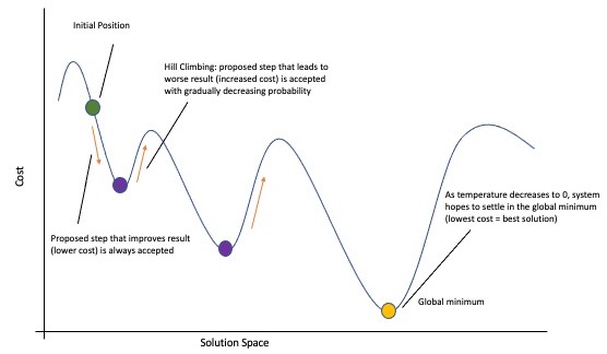
Figure 4. Cartoon schematic of a simulated annealing solver. See the text for more details, but in short: the algorithm is initialized in some starting position (green dot), then a step is taken with some probability (purple dot, red arrow). This repeats until algorithm convergence or a number of iterations is reached.

We complement our QBSolv results with the (classical) simulated annealing implementation provided in D-wave’s neal package; our experiments were run on Amazon Braket notebook instances. Simulated annealing is a stochastic search algorithm that iteratively searches the solution space in the hopes of arriving at the global minimum.

The internal dynamics of SA are governed by the annealing schedule, with corresponding temperature parameter T. This artificial temperature first starts high and cools down towards zero as the algorithm progresses. In doing so, the algorithm shifts from accepting worse (i.e. cost-increasing) moves with higher probability to accepting them with near-zero probability, thereby gradually shifting its optimization mode from exploration to exploitation. By accepting potentially worse moves, simulated annealing can climb cost “hills”, thereby allowing it to (potentially) move out of local minima and search more of the solution space. The high temperature allows the algorithm to be more exploratory at first, then cool towards regions of low cost, generally driving towards regions of low cost, and ideally to the global minimum (e.g. the ground state). Figure 4 provides a depiction of this in a low-dimension space. For more details we refer to an in-depth description of general simulated annealing as can be found in [9, 10].

Benchmarking results

All datasets were generated by the BMW team using custom logic that is implemented in the Robot Operating System (ROS) framework [14]. To be able to calculate the relevant cost values (measured in seconds) to move between nodes and build the corresponding cost matrix W, the physical robot cell is modeled in ROS. This includes loading and positioning of the robot model, importing static collision objects and parsing the robotic objectives. The generation of the data set is then done in two steps. First, a reach-ability analysis is carried out to inspect the different possibilities of applying sealant to a given seam. Second, the motion planning is carried out to obtain the trajectories for all possibilities to move from one seam to all possibilities of processing any other seam. Collision avoidance and time parameterization are included in this process. To this end we adopted the RRT* motion planning algorithm [15]. If the motion planning does not succeed, no (weighted) edge is entered in the motion graph.

Results – Benchmarks

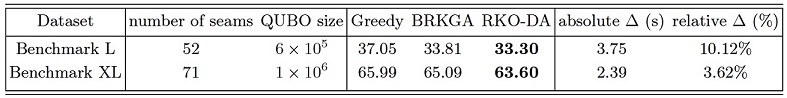
Table 1. Results on key benchmark datasets L (52 seams) and XL (71 seams). We compare BRKGA and RKO-DA to the greedy algorithm as baseline, reporting the raw cost results (in seconds) and the absolute and relative improvement of the best solution (RKO-DA in both cases) against the greedy.

We compare three different algorithmic strategies on these benchmark instances, including BRKGA and RKO-DA (both based on the random-key formalism, but following different optimization paradigms), as well as a greedy baseline. Here we do not provide results for any QUBO-based solution strategies, because these instances are out of reach for QUBO solvers, with approximately ~ 6*10⁵ and 10⁶ binary variables, respectively. Note that numerical results based on the QUBO formalism will be provided later. Hyperparameter optimization for the BRKGA and RKO-DA solvers is done as outlined in [16] using Bayesian optimization techniques. The greedy algorithm was run 10⁴ times, each time with a different random starting configuration, thereby effectively eliminating any dependence on the random seed. We have observed convergence for the best greedy result after typically ~10³ shots, and only the best solutions found are reported. Our results are displayed in Table 1. We find that both BRKGA and RKO-DA outperform the greedy baseline. Specifically, BRGKA yields an improvement of 3.24s (8.74%) on benchmark L and 0.90s (1.36%) on benchmark XL, while RKO-DA yields an even larger improvement of 3.75s (10.12%) on benchmark L and 2.39 (3.62%) on benchmark XL. These improvements can directly translate into cost savings, increased production volumes or both.

Results – Scaling

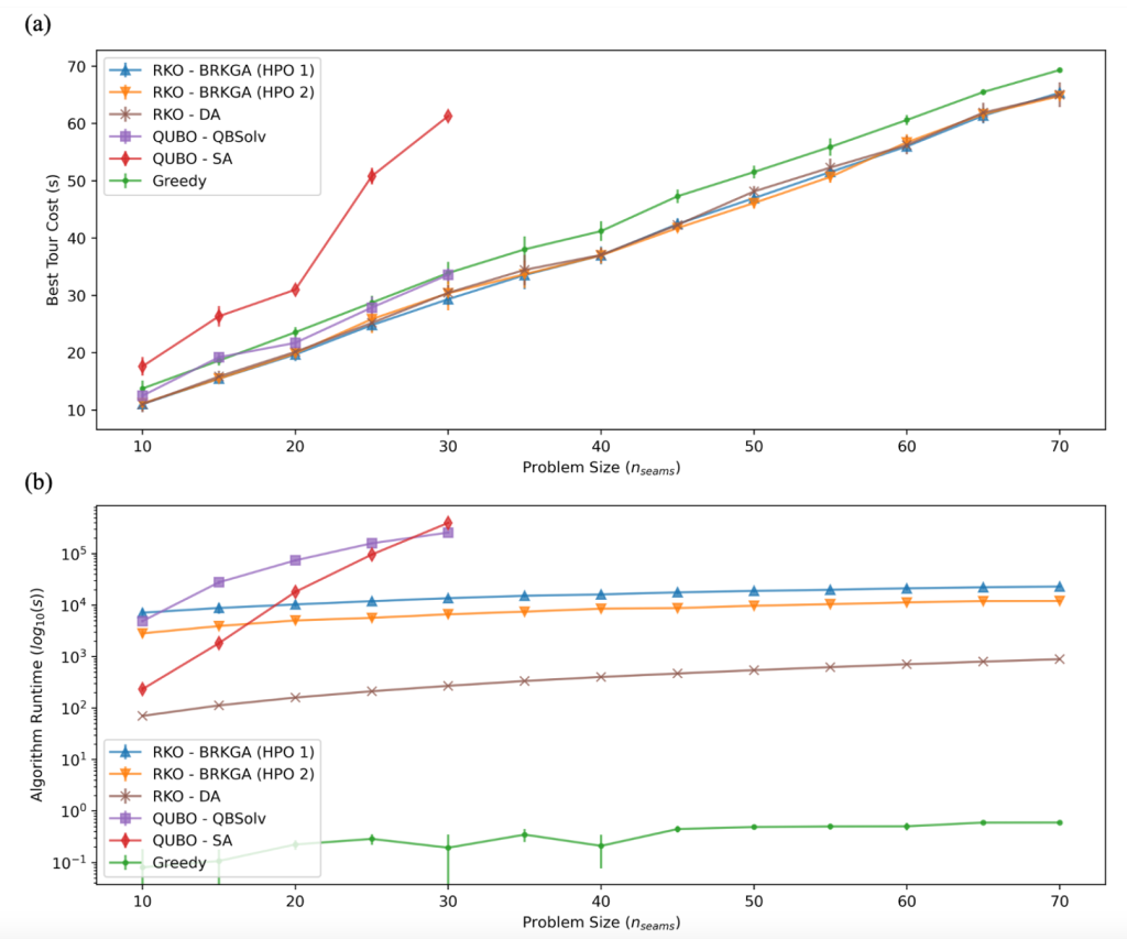
Figure 5. Scaling results used to compare solver quality and runtime across a range of problem sizes, plotting the bootstrapped mean and errors. (a) Solution quality (i.e. solution cost) against problem size. Solvers BRKGA (HPO1 and HPO2) and RKO-DA consistently outperform the greedy benchmark across the full range. QUBO – QBSolv remains competitive with greedy throughout the range it can handle, but is unable to scale to the full range. QUBO – SA remains noncompetitive in the same range as QBSolv. (b) Runtime is plotted for all solvers, in seconds, on a log10 scale. We see that greedy is the fastest without any close competition. RKO-DA is next fastest, with RKO-BRKGA roughly 1.5-2 orders of magnitude slower. Both RKO solvers exhibit a linear runtime scaling in the range. Finally, while QUBO-QBSolv and QUBO-SA exhibit competitive run times at small problem sizes, they suffer from exponential scaling with problem size, and can take a day to complete running at n_seams = 30.

To complement our benchmark results, we performed systematic experiments on datasets with variable size, ranging from n_seams=10 to n_seams=70 in increments of five seams, with ten samples per system size. Our results are displayed in Figure 5, with every curve referring to one fixed set of hyper-parameters (such as population size p, mutant percentage p_m, etc. in the case of BRKGA). We also report numerical results based on the quantum-native QUBO formalism, using both classical simulated annealing, as well as a hybrid (quantum-classical) solver qbsolv.

In Figure 5 (a) We compare results achieved with BRKGA for two sets of hyper-parameters, and for RKO-DA with one set of hyper-parameters, and find that these consistently outperform greedy baseline results, providing about ~10% improvement for real-world systems with n_seams ~ 50. Note that BRGKA (HPO 2) was run with ten shots for problem sizes 45, 50, 55, and 70 to reduce variance observed when using fixed hyper-parameters. Performance of RKO-DA is found to be competitive with BRKGA throughout the range of problem sizes. The QUBO-SA solver is found to be the least competitive, and the least scalable, unable to solve problems beyond n_seams ~ 30. Finally, the QUBO-QBSolv approach performs on par with the greedy algorithm, albeit at much longer run times, but is unable to scale beyond n_seams ~ 30.

Next, we report on the average run times of each solver as a function of problem size; see Figure 5 (b). Unsurprisingly, the greedy algorithm is found to be the fastest solver, taking under a second (~0.60s) to solve the largest problem instances with n_seams=70, after loading in the requisite data. Our implementation of the random-key optimizer RKO-DA can solve the largest problem instances within ~15 minutes, and exhibits a benign, linear runtime scaling with problem size. Our implementation of BRKGA displays a similar scaling, but typically takes a few hours to complete, with average run times ranging from ~0.78 h (HPO 2, n_seams=10) to ~6.40 h (HPO 1, n_seams=70). The observed difference in run times between BRKGA (HPO 1) and BRKGA (HPO 2) can be largely attributed to the different population sizes (with p=9918, and p=7978 for HPO 1 and HPO 2, respectively) and patience values (with patience=52, and patience=66 for HPO 1 and HPO 2, respectively).

Conclusion

In this post we review the results of our collaboration with the BMW Group to solve robot trajectory planning problems at industry-relevant scales, and investigate the potential benefit of applying quantum computing to the problem. We explore two formulations of the problem, a native one based on random keys as well as a quantum-native one based on the QUBO formalism. We apply a variety of solvers to those formulations, including a quantum annealer via D-Wave’s Advantage 4.1 machine, and a simulated annealing solver. We show that the quantum approach, i.e., the QUBO formulation, could not scale to industry-relevant problem sizes, whereas our novel RKO solver was able to outperform all other solvers consistently, yielding up to a 10% improvement over the baseline on real datasets.

For further technical details on this work, see our recently published paper on arXiv and our talk at reMARS 2022. By pursuing a hybrid engagement model including both quantum and classical approaches, customers like the BMW Group are able to grow expertise with quantum computing for the future while also delivering on a classical solver that can yield business-relevant results in the near term. If your company deals with similar motion planning and optimization problems and is looking for novel ways to solve them, we encourage you to reach out to the Amazon Quantum Solutions Lab to start a conversation.

References

1. Muradi and R. Wanka, in 2020 6th International Conference on Control, Automation and Robotics (ICCAR) (2020), pp. 130–138.
2. Lucas, Ising formulations of many NP problems, Front. Physics 2, 5 (2014).
3. Kochenberger, J.-K. Hao, F. Glover, M. Lewis, Z. Lu, H. Wang, and Y. Wang, The Unconstrained Binary Quadratic Programming Problem: A Survey, Journal of Combinatorial Optimization 28, 58 (2014).
4. Glover, G. Kochenberger, and Y. Du, Quantum Bridge Analytics I: A Tutorial on Formulating and Using QUBO Models, 4OR 17, 335 (2019)
5. Anthony, E. Boros, Y. Crama, and A. Gruber, Quadratic reformulations of nonlinear binary optimization problems, Mathematical Programming 162, 115 (2017).
6. F. Gonçalves and M. G. C. Resende, Biased random-key genetic algorithms for combinatorial optimization, Journal of Heuristics 17, 487 (2011)
7. C. Bean, Genetic algorithms and random keys for sequencing and optimization, ORSA Journal on Computing 6, 154 (1994).
8. Virtanen, R. Gommers, T. E. Oliphant, M. Haberland, T. Reddy, D. Cournapeau, E. Burovski, P. Peterson, W. Weckesser, J. Bright, et al., SciPy 1.0: Fundamental
   Algorithms for Scientific Computing in Python, Nature Methods 17, 261 (2020).
9. Tsallis and D. A. Stariolo, Generalized simulated annealing, Physica A: Statistical Mechanics and its Applications 233, 395 (1996), ISSN 0378-4371
10. Xiang, D. Sun, W. Fan, and X. Gong, Generalized simulated annealing algorithm and its application to the thomson model, Physics Letters A 233, 216 (1997),
    ISSN 0375-9601
11. Kadowaki and H. Nishimori, Quantum annealing in the transverse Ising model, Phys. Rev. E 58, 5355 (1998)
12. Farhi, J. Goldstone, S. Gutmann, J. Lapan, A. Lundgren, and D. Preda, A quantum adiabatic evolution algorithm applied to random instances of an NP-complete problem, Science 292, 472 (2001).
13. V. Isakov, G. Mazzola, V. N. Smelyanskiy, Z. Jiang, S. Boixo, H. Neven, and M. Troyer, Understanding Quantum Tunneling through Quantum Monte Carlo Simulations, Phys. Rev. Lett. 117, 180402 (2016).
14. Quigley, K. Conley, B. P. Gerkey, J. Faust, T. Foote, J. Leibs, R. Wheeler, and A. Y. Ng, Ros: an open-source robot operating system, https://ros.org
15. Karaman and E. Frazzoli, Sampling-based algorithms for optimal motion planning, The International Journal of Robotics Research 30 (2011).
16. Bergstra, D. Yamins, and D. Cox, in Proceedings of the 30th International Conference on Machine Learning, edited by S. Dasgupta and D. McAllester (PMLR, Atlanta, Georgia, USA, 2013), vol. 28 of Proceedings of Machine Learning Research, pp. 115–123