Reservoir computing on an analog Rydberg-atom quantum computer

This post shows how quantum reservoir computing (QRC) can tackle machine learning challenges using Rydberg-atom quantum computers. Readers will learn how QRC works, see its performance on image classification and time series prediction tasks, and understand when it outperforms classical methods—particularly for small datasets in pharmaceutical research. After decades of progress, machine learning (ML) has become a foundation of modern technology, powering applications in areas such as computer vision, financial market prediction, and natural language processing. Despite these advances, ML still struggles with problems of growing scale and complexity. To overcome these limitations, there has been growing interest in exploiting the principles of quantum mechanics to design quantum machine learning (QML) algorithms to tackle ML problems such as image classification or those involving quantum data [1]. Among the many QML approaches proposed, quantum reservoir computing (QRC) has emerged as a promising approach for implementation on near-term quantum hardware [2-6].

In this post, we dive deep into recent research done by QuEra Computing and collaborators on QRC [7,8]. Ref. [7] presents a quantum reservoir learning algorithm using Rydberg-atom quantum computers for machine learning tasks. The authors implemented the algorithm experimentally for various tasks such as image classification and time series prediction. The algorithm was subsequently applied numerically in Ref. [8] to gauge the performance of QRC for molecular property learning. The authors observed robust QRC performance on small datasets relevant for pharmaceutical research. Interested readers can reproduce the results on Amazon Braket by following the authors’ tutorials [9, 10].

Classical reservoir computing

Reservoir computing is a machine learning paradigm, where the relation between input signals and outputs is modeled by the time dynamics of a non-linear system with fixed parameters called a reservoir. The reservoir maps the input to a high-dimensional space, known as the configuration space of the reservoir, then a readout layer is trained to characterize the time-dependent states of the reservoir and map it to the desired output. Compared to other machine learning methods, one benefit of reservoir computing is that only the readout layer requires training while the reservoir parameters remain fixed, resulting in low training cost. Additionally, reservoir computing is amenable to analog hardware implementations, either classical or quantum, enabling access to the inherent computational capabilities of diverse physical systems [11-13].

As an example of classical reservoir computing (CRC), we consider classifying the Modified National Institute of Standards and Technology (MNIST) images of handwritten digits using a chain of N_q classical spins. Each spin is described by a time-dependent vector S_i(t) = [S^x_i(t), S^y_i(t), S^z_i(t)] where 1 ≤ i ≤ N_q labels the spins. To encode an image, we convert it into a N_q-dimensional feature vector x (0 ≤ x_i ≤ 1) and set the site-dependent longitudinal magnetic field as Δ_i = Δ^maxx_i. With that, we have set up a reservoir whose dynamics are determined by the features of the image. We then sample observables from the evolution of the reservoir, such as the Z-component of all spins S^z_i(t) and the correlation functions S^z_i(t)S^z_j>i(t), which yield a data-embedding vector. Finally, we build such data-embedding vectors for all images and train a linear readout (e.g., linear regression) to perform classification.

Quantum Reservoir Computing with Rydberg atoms

From the preceding example, we see that a reservoir can be viewed as a programmable analog computer that is used as a subroutine to perform a given machine learning task. The classical spin chain is not the only choice for the reservoir, and a natural alternative is a quantum spin system, which can be viewed as an analog quantum computer. In Ref. [7], the authors considered an analog quantum computer based on Rydberg atoms and implemented a QRC algorithm utilizing the quantum dynamics of the system.

Overview

The QRC algorithm workflow is summarized in Figure 1. Like its classical counterpart described earlier, it consists of three steps. The algorithm starts by converting the input data, whether an image for classification or a time series for prediction, into a feature vector readily encoded to a two-dimensional Rydberg system. Each Rydberg atom is a two-level system with tunable position r_i and is subject to a local detuning Δ_i(t), which is analogous to the site-dependent longitudinal magnetic field used in the CRC example, and a global detuning Δ(t), analogous to a uniform longitudinal magnetic field. After the feature vector is encoded into these parameters, in the second step, the system then evolves over varying time periods and can be probed by measuring a set of local Pauli-Z observables including <Z_i(t)> and <Z_i(t) Z_j>i(t)>. These observables form the data-embedding vectors in a high dimensional space where linear separability becomes prominent. Hence, one can use the data-embedding vectors to train a simple classification model, such as a support vector machine (SVM), in the last step of the workflow.

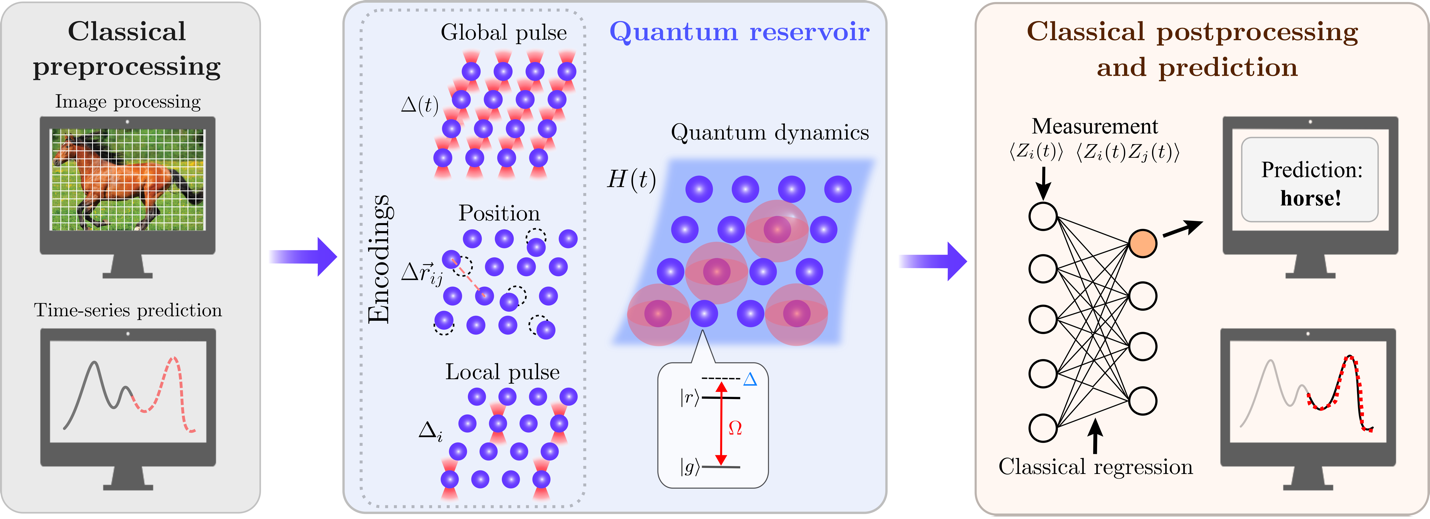
Figure 1 – Overview of the QRC algorithm with Rydberg atoms.

Although QRC shares the same workflow as CRC, using quantum systems as reservoirs enables access to a state space beyond product states and enables long-range quantum correlations that are unavailable classically. As a result, QRC can take advantage of the superposition and entanglement unique to quantum systems to tackle challenging machine learning tasks with data of increasing complexity and intricate patterns.

Classification

In Ref. [7], the authors applied the QRC algorithm to the MNIST classification task by encoding images into either the positions or the local detunings of atoms in a chain. Here we focus on the former method. For two atoms with positions r_i and r_j, the interaction strength between them is given by

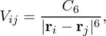where  is the Rydberg interaction constant. The atoms in the chain are initialized to be uniformly separated by a distance d, and we use position encoding to modulate the atom positions such that the interaction between neighboring atoms reads

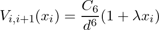
Here  is a task-dependent encoding scale. Once the atom arrangements are determined, the Rydberg system then evolves (for five successive timesteps), after which we measure the time-dependent observables. This process is repeated for all images in the training set, and an SVM is trained with all the measured observables.

The test accuracy of the QRC algorithm using position encoding is shown in Figure 2, where the authors compare the performance of QRC with other machine learning methods for the 3/8-MNIST binary classification task. The simulations and experiments are carried out using a chain with nine atoms. The exact simulation of QRC shows similar accuracy in predicting the downscaled images in the test set compared to CRC simulation and a four-layer feedforward neural network (NN). The authors also compare the test accuracy from a linear SVM, which is obtained by removing the reservoir from the workflow (see Figure 1) and training the SVM directly with the feature vectors. The relatively poor performance of the linear SVM illustrates the critical role of introducing nonlinearity via the reservoir, either classical or quantum, in the algorithms.

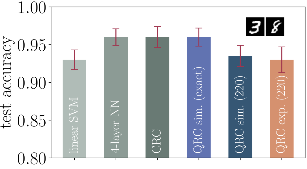
Figure 2 – Comparison of the performance of QRC with other machine learning methods for 3/8-MNIST binary classification task.

The authors also consider a different classification task: classifying tomato diseases based on leaf images. Instead of using a one-dimensional chain of atoms, position encoding is applied to a two-dimensional atom array, as shown in Figure 3(a). In this setup, each of the up to N_q = 108 atoms represents a pixel in the downscaled image. As noted, the performance of the QRC algorithm improves when more atoms are used in the encoding. This is indeed the case as shown in Figure 3(b). Although the four-layer NN (with ~20,000 hidden parameters) shows better overall performance than QRC for most of the range of N_q considered, QRC shows better scaling with respect to the number of atoms used in the encoding. Upon increasing the number of shots per datapoint from 100 to 400, the QRC test accuracy improves significantly across all system sizes and reaches similar performance as the four-layer NN for N_q ≥ 90. Note that there are known classical methods outperform the linear SVM or four-layer NN used in the benchmark. Therefore, the proof-of-concept results obtained here do not indicate that QRC performs better than NN or other state-of-the-art classical machine learning methods.

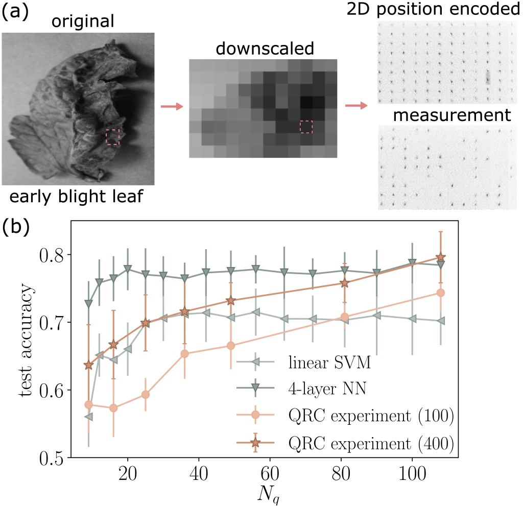
Figure 3 – QRC for classifying tomato diseases based on leaf images. (a) Illustration of 2D position encoding. (b) Comparison with other machine learning methods. Here Nq corresponds to the number of pixels in the downscaled image.

Time series forecasting

Because the computational power of reservoir computing comes from the time dynamics of physical systems, it is natural to apply the framework to problems such as time series prediction. In such applications, reservoir computing, which can be viewed as a special case of recurrent neural networks, uses the time dynamics of one physical system to simulate that of another physical system [11-13]. Guided by such intuition, the authors apply the QRC algorithm to a time series forecasting task in Ref. [7], where they study all the encoding methods listed in Figure 1. Here, we describe in more detail the encoding method with global detuning.

The time series forecasting task considers the light intensity of a laser in the chaotic regime, as shown in Figure 4(a). Time points between 1000 and 1400 are used as a training set, and subsequent time points are used as a test set. The authors preprocess the training data by moving a sliding window of length N_s across it. In each window the feature vector is defined as x=[l_k, l_k+1, …, l_k+Ns-1], where l_j is the intensity value at the j-th time point. This is the so-called one-step prediction task. They then use the feature vector to define the global detuning at different time points as Δ(t_i)= Δ^maxx_i, as illustrated in Figure 4(a), which controls the dynamics of the Rydberg atoms. The same process is repeated for subsequent sliding windows to obtain a data-embedding vector for training the final readout layer. With global detuning encoding, the authors use a chain with N_q atoms that are equally separated from each other. It is important to note that the encoding capability of global detuning encoding is independent of the number of atoms (N_q), which is in sharp contrast to the other two encoding methods. The impact of such a difference to their prediction accuracies is shown in Figure 4(b).

The results of the time series forecasting task are shown in Figure 4(b), which compares the three different QRC encodings, for both simulation and experiments. The metric normalized mean-square error (NMSE), quantifies the discrepancy between the predicted and true time series in the test set, and lower values of NMSE mean better prediction accuracies. We can see that encoding with global detuning (labeled as “pulse”) performs worse than the other two encoding methods, position and local, in both simulation and experiments. This is not surprising because the position and local encoding methods provide higher degrees of control for the Rydberg system which results in a reservoir with a more complex configuration space and higher expressibility. The encoding capacity of global detuning is limited by thermalization, a constraint not present in the other encoding methods. Interested readers can find more on the differences in these encoding methods in Refs. [3] and [7].

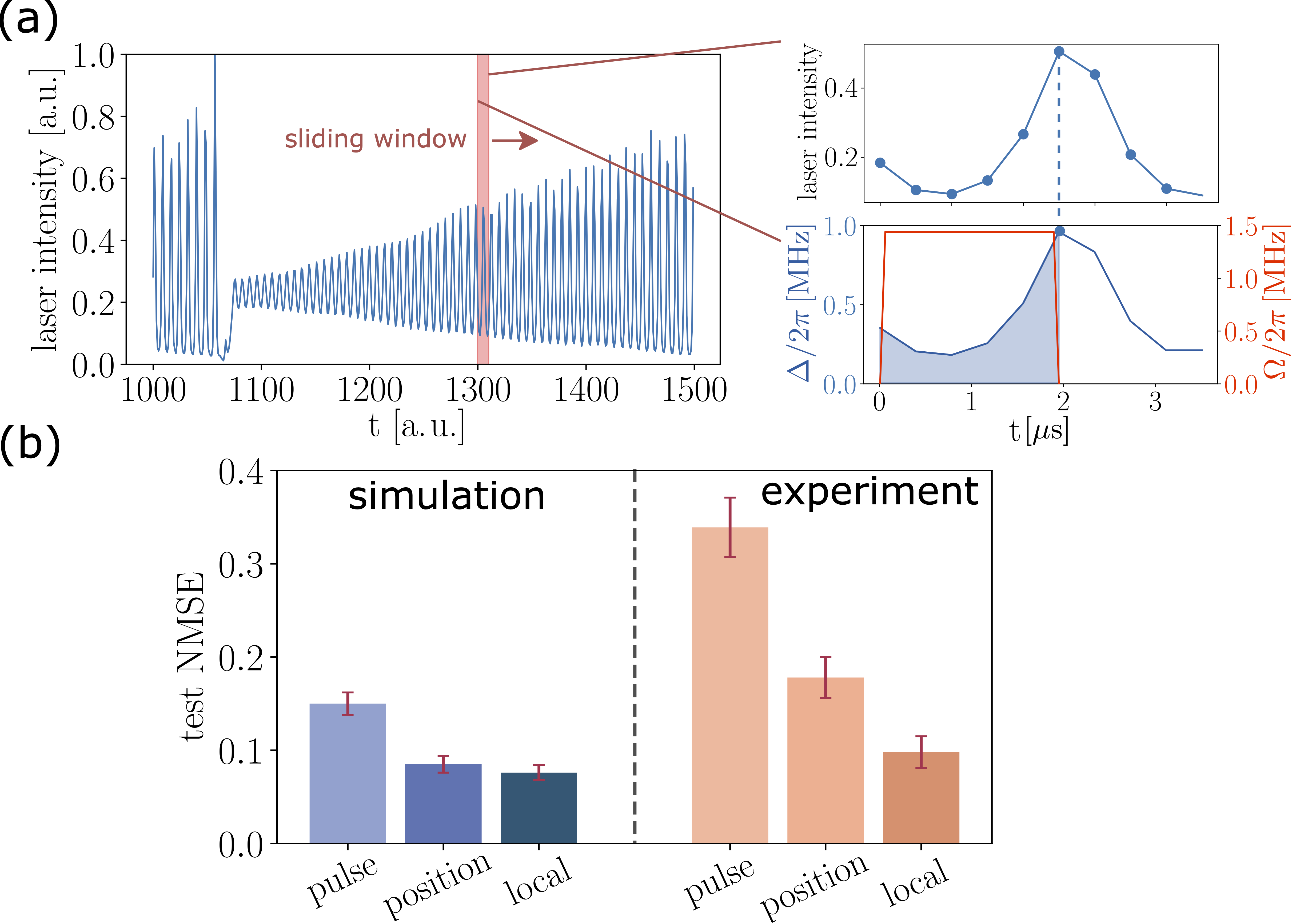
Figure 4 – Performance of QRC for time series forecasting. (a) Illustration of feature vector construction with Ns=9. (b) Comparison of three encoding methods for both simulation and experiment (lower is better).

Comparative quantum kernel advantage

In Ref. [7], the authors also discuss the comparative quantum kernel advantage of QRC for a certain synthetic dataset. They consider QRC as a kernel and apply the quantum kernel method to the 3/8-MNIST binary classification task, followed by retraining and testing the QRC and CRC with the obtained synthetic dataset. Despite the synthetic nature of the resulting dataset, the experiment shows the existence of a dataset for which QRC exhibits better test accuracy compared to CRC.

Remarks on the effects of experimental noise

In Ref. [7], the authors also discuss extensively the effects of experimental noise on the QRC algorithm. For example, the difference between the local pulse and position encodings shown in Figure 4(b) can be partially attributed to the shot-to-shot atom position fluctuations. Although these fluctuations are present for all experiments, the position encoding is more susceptible to such noise. Further, quantum dynamics tends to thermalize in the long-time limit, for both the global and local pulse encodings, and this could cause a significant fraction of the feature vector to be encoded in a lossy manner. Ref. [7] provides extensive simulations showing parameter regimes where QRC performs robustly despite noise.

Robust Quantum Reservoir Computing for Molecular Property Prediction

In Ref. [8], the authors explore a separate application of QRC in pharmaceutical research: predicting molecular properties from a set of chemical descriptors. They numerically simulate QRC and compare its performance to classical machine learning methods using the Merck Molecular Activity Challenge datasets (MMACD). Their findings suggest that QRC performs better than classical methods when the training dataset is limited, which could be valuable for pharmaceutical applications. Using uniform manifold approximation and projection (UMAP) analysis, the QRC-embedded data exhibits clearer clustering patterns related to molecular activity, demonstrating that quantum reservoir embeddings appear more interpretable in lower dimensions. The research indicates that QRC-enhanced models may offer advantages in biomedical data science, particularly for cases that have small training sets and require interpretable, robust models.

The comparison of the performance of QRC and various classical methods are shown in Figure 5. In Figure 5(a), the predictive abilities of the methods are quantified with mean squared error (MSE, smaller is better). The MSE of classical baselines rises steeply as the number of training records decreases, while the QRC embeddings—particularly with two-body observables (labeled as “QRC Embedding” for clarity)—retain comparatively low MSE even at 100 samples. This indicates that QRC performance deteriorates more slowly under data scarcity. Figure 5(b) compares the UMAP 2D projections for the classical reservoir embedding and QRC embedding (with two-body observables). Molecular activity labels for the former method are intermixed with weak cluster separation, making activity patterns hard to distinguish. By contrast, the same labels for QRC form clearer, more compact clusters, indicating that QRC embeddings yield more interpretable, low-dimensional representations that better reflect molecular activity.

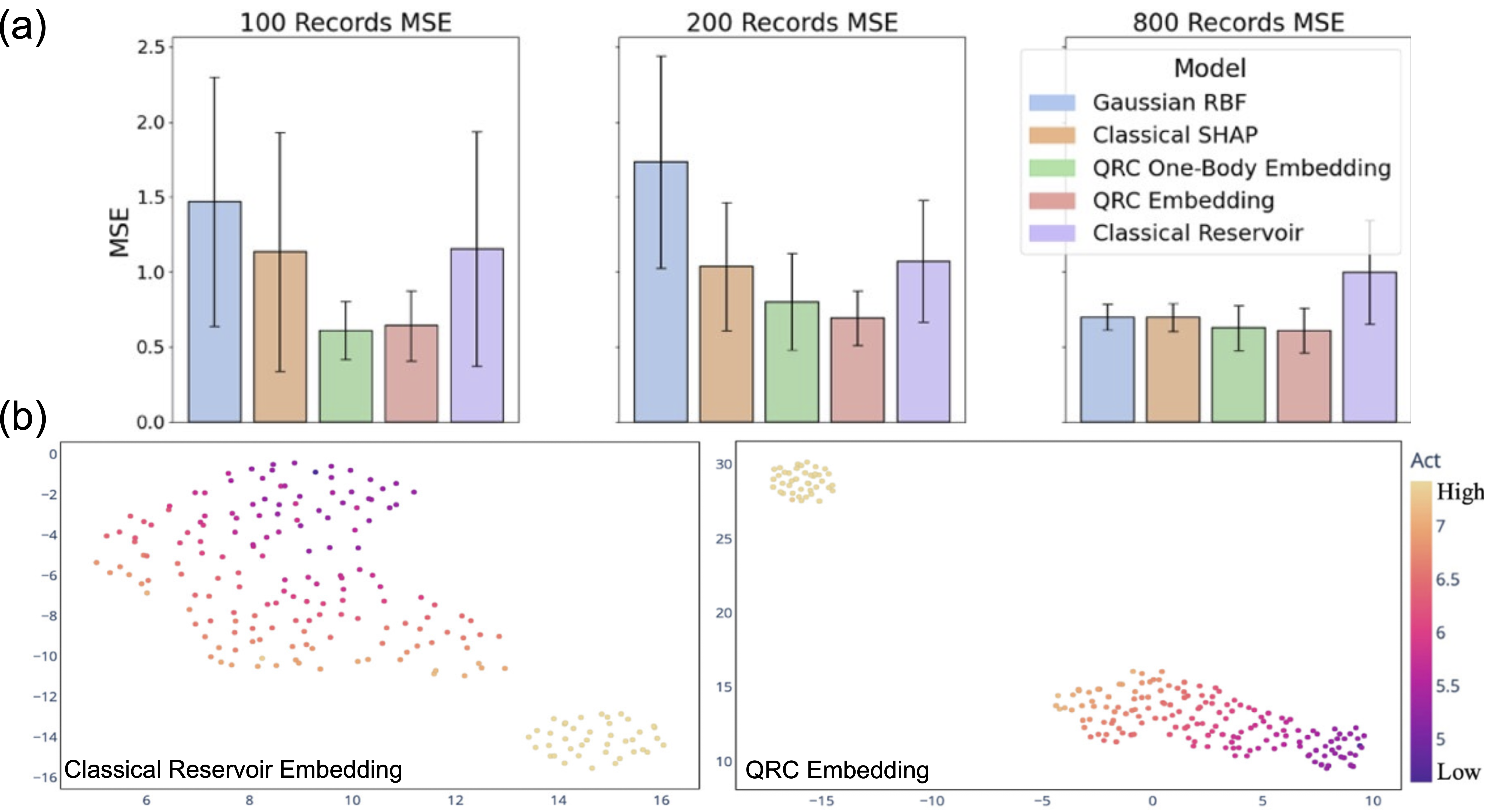
Figure 5 – Comparison of performances of QRC and classical methods for molecular property prediction. (a) Comparison for the performance on a MMACD dataset. (b) Comparison UMAP 2D projections.

Conclusion

This research demonstrates that quantum reservoir computing on Rydberg-atom systems can match or exceed classical methods for specific ML tasks, particularly when training data is limited. Readers working with small datasets in pharmaceutical research or need interpretable models may find in QRC advantages worth exploring. At Amazon Braket, we aim to enable researchers to more easily test their algorithms and make the most out of various quantum devices. To get started with Amazon Braket, refer to our example notebooks. Researchers from accredited institutions can apply for credits by submitting a research proposal here.

References

[1] D. García, et al. (2022). Systematic Literature Review: Quantum Machine Learning and its applications. Computer Science Review 51, 100619 (2024).

[2] K. Fujii, et al. (2016). Harnessing disordered ensemble quantum dynamics for machine learning. Physical Review Applied 8, 024030 (2017).

[3] R. Bravo, et al. (2022). Quantum Reservoir Computing Using Arrays of Rydberg Atoms. PRX Quantum 3, 030325.

[4] J. Dudas, et al. (2022). Quantum reservoir neural network implementation on coherently coupled quantum oscillators. npj Quantum Information 9, 1, 64 (2023).

[5] T. Yasuda, et al. (2023). Quantum reservoir computing with repeated measurements on superconducting devices. arXiv: 2310.06706.

[6] P. Mujal, et al. (2021). Opportunities in quantum reservoir computing and extreme learning

machines. Adv. Quantum Technol. 2100027 (2021).

[7] M. Kornjača, et al. (2024). Large-scale quantum reservoir learning with an analog quantum computer. arXiv: 2407.02553.

[8] D. Beaulieu, et al. (2024). Robust Quantum Reservoir Computing for Molecular Property Prediction. Journal of Chemical Information and Modeling 65, 16, 8475 (2025).

[9] https://github.com/QuEraComputing/QRC-tutorials

[10] https://github.com/QuEraComputing/robust-qrc-molecular-prediction

[11] H. Jaeger (2010). The “echo state” approach to analysing and training recurrent neural networks. GMD Report 148, German National Research Center for Information Technology, 2001.

[12] W. Maass (2011). Liquid State Machines: Motivation, Theory, and Applications. Computability in Context. February 2011, 275-296.

[13] G. Tanaka, et al. (2019). Recent advances in physical reservoir computing: A review. Neural Networks, 115, 100 (2019).