How to attribute Amazon Redshift costs to your end-users

Amazon Redshift is a fast, fully managed cloud data warehouse that makes it simple and cost-effective to analyze all your data using standard SQL and your existing business intelligence (BI) tools. In this two-part series, we discuss how to attribute Amazon Redshift costs at the user and group level.

When using Amazon Redshift, you can choose either of the two pricing models available: On-Demand pricing and Reserved Instance pricing.

On-Demand pricing allows you to pay for capacity by the hour with no commitments and no upfront costs; you simply pay an hourly rate based on the type and number of nodes in your cluster. Partial hours are billed in 1-second increments following a billable status change such as creating, deleting, pausing, or resuming the cluster.

Reserved Instances are appropriate for steady-state production workloads, and offer significant discounts over On-Demand pricing.

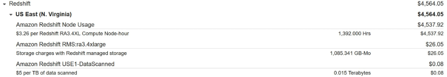
At the end of billing cycle, you see an itemized billing of your usage of AWS Services, as in the following screenshot.

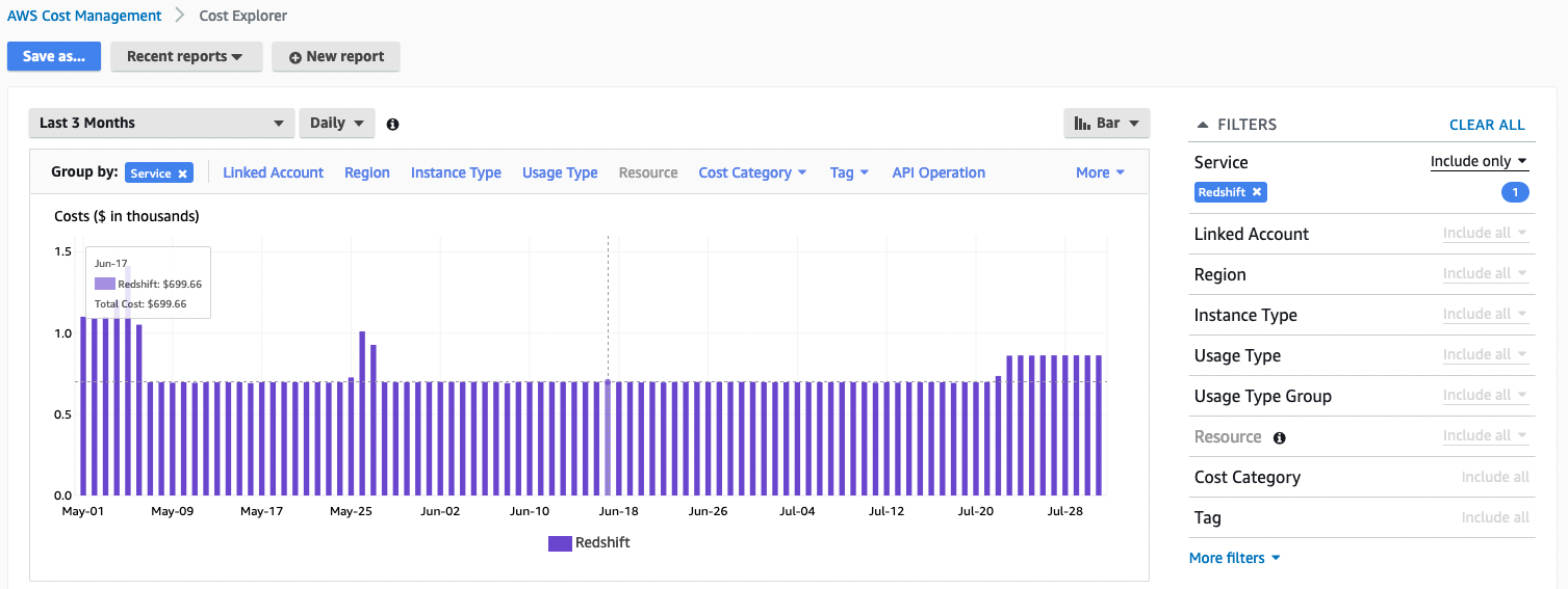
In addition, you can check AWS Cost Explorer for further details on the cost. For example, the following screenshot shows usage cost for Amazon Redshift per day.

These views give you the overall cost of using Amazon Redshift. However, you may need to attribute the cost at the user or group level. For example, what’s the usage cost in Amazon Redshift by the finance business unit?

Use case

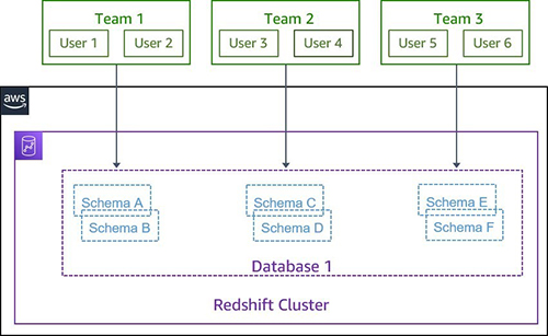
Amazon Redshift allows you administer controls to individual objects by users and groups. You can use schemas to group database objects under a common name, which provides a convenient way to manage access, rather than by individual objects. Organizations typically organize related objects in schemas. For example, a finance_schema contains all the related objects related to the finance dataset, and granting access to the finance schema to the finance_group allows only users who are members of the finance_group to access this dataset.

The following diagram illustrates this schema-based setup.

Typically, you can also grant a schema access to multiple groups (teams) or individual users. For example, a finance user might want access to sales data to perform the annual budgeting, or you may have common datasets like the customer information that can be shared by different groups. The following diagram illustrates this setup.

Now, the goal of the cost attribution involves proportional assignment of the overall cost to the individual groups or users.

Cost attribution

At its simplest form, cost attribution can be determined using the amount of the storage assigned to the individual objects using the ownership of the objects to the groups. But the downside of this approach is it doesn’t provide a true translation of the resource usage. For example, let’s say Team 1 has total object size of 1 TB, whereas Team 2 has 100 GB in total size. Team 1 member runs 10 queries daily, and Team 2 runs 1,000 queries per day. Of course, Team 2 uses more resources than Team 1.

The Amazon Redshift RA3 architecture allows you to pay for the compute and data warehouse storage capacity separately, therefore storage doesn’t reflect the resources used by the teams for the cost attribution.

Cost attribution model

The methodology for the cost attribution model has to be translated to the resource used by the user or team. The SQL queries used to create and manipulate database objects, run queries, load tables, and modify the data provide an ideal mechanism to associate the resource of the data warehouse. The following table shows a matrix of possible different query metrics that you can use to associate cost attribution.

You can now derive a costing model using these deterministic metrics as follows:

Overall query cost = (query data scan cost * data scan weighted score) + (Query CPU cost * CPU weighted score) + (query run cost * run weighted score) + Redshift Spectrum cost

With the preceding model, you can now associate the query cost per user, which can be rolled up to individual teams (or groups) for cost attribution.

Use Amazon Redshift system tables for cost attribution

Amazon Redshift system tables contain information about how the system is functioning and logs user activities. You can use the following system tables to capture deterministic metrics:

• svl_s3query_summary – Shows a summary of all Redshift Spectrum queries (Amazon Simple Storage Service queries) that have been run on the system
• stl_wlm_query – Shows the attempted run of a query in a service class handled by WLM
• stl_query – Shows run information about a database query
• svl_qlog – Shows a log of all queries run against the database
• stl_alert_event_log – Shows an alert when the query optimizer identifies conditions that might indicate performance issues

We used these system tables to create the following views, which are available in the GitHub repo:

• redshift_spectrum_scan_summary_vw
• redshift_query_summary_vw
• redshift_query_attribution_vw

We used the following representative query to obtain the metrics that can be used for the cost attribution:

SELECT trim(to_char(rqs.event_date_utc, 'Day')) AS metric_day_of_week
      ,rqs.event_date_utc
      ,rqs.database_name
      ,rqs.queue_name
      ,rqs.db_username
      ,COUNT(1)                                                                                      AS query_count
      ,SUM(rqs.query_cpu_time_secs)                                                                  AS cpu_time_secs
      ,SUM(case when rqs.used_concurrency_scaling = 0 then rqs.query_execution_time_secs else 0 end) AS execution_time_secs
      ,SUM(rqs.query_blocks_read_mb) + SUM(rqs.query_temp_blocks_to_disk_mb)                         AS disk_io_mb
      ,SUM(rqs.rated_spectrum_scan_size_mb)                                                          AS rated_spectrum_scan_size_mb
FROM redshift_query_summary_vw rqs
GROUP BY trim(to_char(rqs.event_date_utc, 'Day'))
        ,rqs.event_date_utc
        ,rqs.database_name
        ,rqs.queue_name
        ,rqs.db_username;

The following table is our sample output (not all columns are shown).

Let’s assume that the total Amazon Redshift incurred cost is $100 per day. If we use a simple data scanned model (total_disk_io_mb), we can attribute cost to individual users, as shown in the following table.

The following query automatically calculates the attribution cost of a query based on the defined cost attribution model, which also includes the spectrum cost (if any):

SELECT TRIM(TO_CHAR(rqa.event_date_utc,'yyyy-mm')) AS metric_month,
       TRIM(TO_CHAR(rqa.event_date_utc,'Day')) AS metric_day_of_week,
       rqa.event_date_utc,
       rqa.database_name,
       rqa.queue_name,
       rqa.db_username,
       MIN(rqa.daily_redshift_compute_cost) AS daily_redshift_compute_cost,
       SUM(rqa.redshift_query_cost) AS total_redshift_query_cost
FROM redshift_query_attribution_vw rqa
GROUP BY TRIM(TO_CHAR(rqa.event_date_utc,'yyyy-mm')),
         TRIM(TO_CHAR(rqa.event_date_utc,'Day')),
         rqa.event_date_utc,
         rqa.database_name,
         rqa.queue_name,
         rqa.db_username;

The following table shows our output (not all columns are shown) for the cost attributed at user level.

To show the compute cost of your own Amazon Redshift cluster, you need to download the redshift_query_attribution_vw view and adjust the numbers on the following columns in the redshift_cluster_node subquery of the view:

• price_per_node_per_hour
• daily_operation_hour
• spectrum_price_per_tb
• concurrency_price_per_second
• cpu_rated_score
• disk_io_rated_score
• execution_rated_score
• daily_redshift_compute_cost

The sum of the cpu_rated_score, disk_io_rated_score, and execution_rated_score should be equal to 1.

System tables retain approximately 2–5 days of log history, depending on log usage and available disk space. If you want to retain the log data, you need to periodically copy it to other tables or unload it to Amazon S3. You can use the Amazon Redshift System Object Persistence Utility for longer persistence.

Conclusion

Amazon Redshift logs deterministic metrics that you can use to associate resource usage of the cluster to a user or team. You can collect these metrics for a fine-grained cost attribution model to meet your business needs.

You can also automate the reports using the Amazon Redshift scheduling feature or through any of your BI tools. With the cost attribution model, you can easily manage the costs of your Amazon Redshift cluster in a fine-grained fashion and identify options for optimization and scaling.

About the Authors

Jason Pedreza is an Analytics Specialist Solutions Architect at AWS with over 13 years of data warehousing experience. Prior to AWS, he built data warehouse solutions at Amazon.com. He specializes in Amazon Redshift and helps customers build scalable analytic solutions.

Bhanu Pittampally is Analytics Specialist Solutions Architect based out of Dallas. He specializes in building analytical solutions. His background is in data warehouse – architecture, development and administration. He is in data and analytical field for over 13 years.

Thiyagarajan Arumugam is a Principal Solutions Architect at Amazon Web Services and designs customer architectures to process data at scale. Prior to AWS, he built data warehouse solutions at Amazon.com. In his free time, he enjoys all outdoor sports and practices the Indian classical drum mridangam.