Optimizing PySpark UDFs on AWS Glue 6.0 with native Arrow UDFs

The AWS Prescriptive Guidance topic Optimize user-defined functions explains that Python UDFs in PySpark can degrade performance because data must be serialized between the Java Virtual Machine (JVM) and the Python runtime. It recommends, in order of preference: use built-in Spark SQL functions, implement UDFs in Scala or Java, or use Apache Arrow-based UDFs (also known as vectorized or pandas UDFs) for vectorized workloads.

That guidance is based on a concise example: the operation a + b over 10 million rows, comparing a standard Python UDF, a vectorized UDF, and Spark SQL. In this post we extend that example to answer a few practical questions we hear from customers:

• Does the ranking hold as data volume grows, from 10 million to 100 million rows?
• Does it hold for a more compute-intensive operation, not only a + b?
• AWS Glue 6.0 (Apache Spark 4.1.1) adds two newer Arrow-based options: the Arrow-optimized Python UDF (useArrow=True) and the native Arrow UDF (arrow_udf, from Apache Spark 4.1.0). Where do they fit relative to a vectorized (pandas) UDF?
• Can we attribute the difference to the data transport, the computation, or both?

We ran each variant as an AWS Glue 6.0 job and share the results, the methodology, and a controlled experiment that clarifies why the vectorized UDF performs the way it does.

Solution overview

We ran a parameterized benchmark harness as an AWS Glue 6.0 job. The job generates a Parquet dataset once, writes it to Amazon Simple Storage Service (Amazon S3), and then runs each UDF variant against the same files, so that every approach reads identical data. We measured across three data volumes (10M, 50M, and 100M rows, where M = million) and three workloads of increasing per-row cost.

The following image shows the workflow of the benchmark.

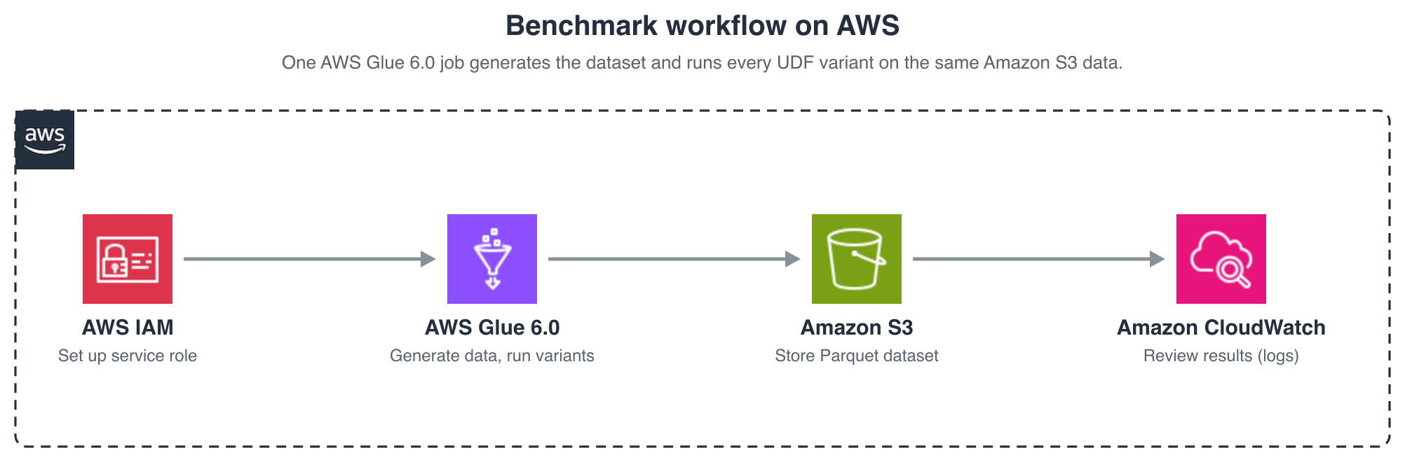
Figure 1: Benchmark workflow running each UDF variant as an AWS Glue 6.0 job

The high-level steps are:

1. Set up the prerequisite AWS Identity and Access Management (IAM) role and Amazon Simple Storage Service (Amazon S3) bucket.
2. Deploy and run the AWS Glue 6.0 job, which generates the dataset and runs the variants.
3. Review the results, emitted to the job logs and optionally written back to Amazon S3.

The approaches we compared

All variants compute the same result. They differ in how data crosses the JVM–Python boundary and how the per-row logic runs.

The vectorized UDF and the Arrow-optimized Python UDF both use Apache Arrow for transport, so both show ArrowEvalPython in the physical plan. The difference is the computation:

• A vectorized UDF (pandas UDF) receives a pandas.Series (a batch of rows), so the computation can be expressed with NumPy and runs on the whole batch in native code. It involves a pandas conversion on top of Arrow.
• An Arrow-optimized Python UDF is a scalar UDF: the function receives one value per call. Arrow makes the transport efficient, but the Python code still runs one row at a time.
• A native Arrow UDF (the arrow_udf decorator, introduced in Apache Spark 4.1 and available in AWS Glue 6.0) receives and returns a pyarrow.Array and computes with PyArrow compute kernels. It operates directly on Arrow data, without the pandas conversion that a vectorized UDF performs.

The following image summarizes how each variant crosses the boundary.

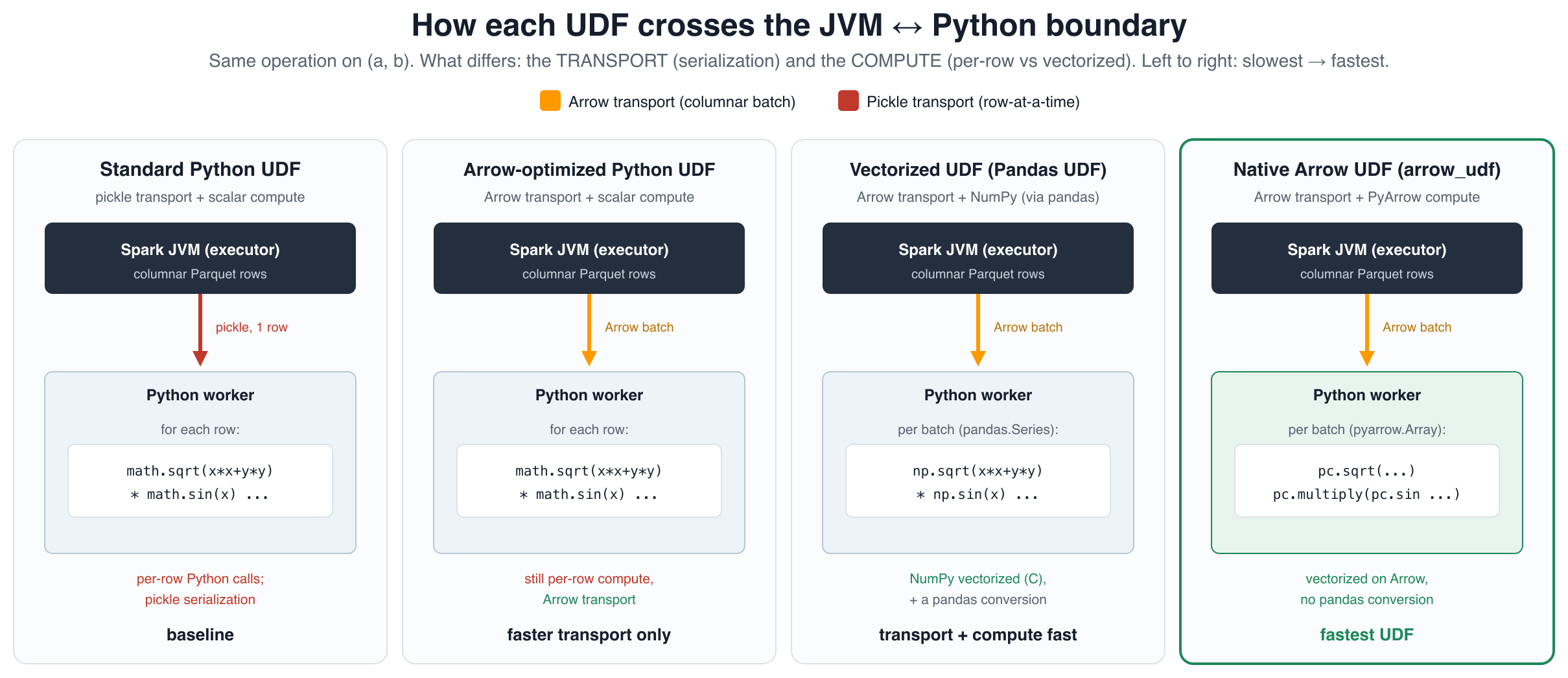
Figure 2: How each UDF variant crosses the JVM to Python boundary

The code difference reflects that distinction. The registration shape is similar, but the computation differs:

# Arrow-optimized Python UDF: scalar function, Arrow transport
op = udf(lambda a, b: math.sqrt(a*a + b*b) * math.sin(a), DoubleType(), useArrow=True)

# vectorized UDF (pandas UDF): batch function, Arrow transport + NumPy computation
@pandas_udf(DoubleType())
def op(a, b):                       # a, b are pandas.Series (a batch of rows)
    return np.sqrt(a*a + b*b) * np.sin(a)

# native Arrow UDF: batch function, Arrow transport + PyArrow compute (no pandas)
@arrow_udf("double")
def op(a, b):                       # a, b are pyarrow.Array (a batch of rows)
    return pc.multiply(pc.sqrt(pc.add(pc.multiply(a, a), pc.multiply(b, b))), pc.sin(a))

Environment and setup

• Runtime: AWS Glue 6.0 (Apache Spark 4.1.1, Python 3.13, Scala 2.13), 10 × G.1X executors plus the driver, in the US East (N. Virginia) AWS Region (us-east-1).
• Data: A Parquet dataset with two bigint columns (a, b), written once to Amazon S3 and read back by every variant so all approaches read identical files.
• Volumes: 10M, 50M, and 100M rows. Two dimensions are combined in every run: the workload (the per-row operation) and the query shape (how that operation is aggregated). Each of the three workloads was run under both query shapes, for every approach and volume.

Workloads (the per-row operation)

We chose three operations of increasing cost, to show how the results change as the per-row work shifts from “almost nothing” to “Python-only.”

The progression matters. arith isolates the transport cost. mathheavy adds real computation, so vectorization can help. All five approaches apply, including the native Arrow UDF, because the math maps onto PyArrow compute kernels. pyheavy is the opposite extreme: an iterative loop that maps onto neither SQL nor PyArrow compute kernels, so Spark SQL and the native Arrow UDF don’t apply and only the Python-based UDFs remain.

Query shapes (how the operation is aggregated)

Each workload is measured under two query shapes, because they exercise different execution paths in the engine:

• Streaming: sum(op(a, b)) — A full scan of every row, reduced to a single value. This isolates the per-row cost with minimal aggregation overhead.
• Stateful: GROUP BY cast(op(a, b) AS bigint) % 1,000,000 — A full scan followed by a high-cardinality aggregation (about one million groups), which adds a shuffle and a large hash table.

Both shapes apply to all three workloads. To keep the tables readable, the following results report the streaming shape. We measured the stateful shape too and found the same ranking, with representative stateful figures given in the Results section.

Methodology

Two decisions had a material effect on the results.

Warm-up and best-of-N. The first run of each variant is dominated by cluster, JVM, and Python worker start-up. We ran one warm-up iteration that we discard, then N timed iterations, and report the best (and mean).

Reading fresh on every iteration. Our first attempt reused a cached DataFrame, and Spark cached the Parquet blocks and pruned the plan for a scalar count(). As a result the UDF timings didn’t scale with data size, and Spark SQL appeared slower than the UDFs. That was the opposite of the expected result. We corrected this by clearing the cache and re-reading the Parquet on every timed iteration, and by using sum(...) so the optimizer can’t prune the per-row work.

def bench(name, fn, repeat, warmup, pre=None):
    for _ in range(warmup):
        if pre: pre()
        fn()                     # discarded
    times = []
    for _ in range(repeat):
        if pre: pre()            # e.g. spark.catalog.clearCache()
        t = time.perf_counter(); fn(); times.append(time.perf_counter() - t)
    return {"best_sec": min(times), "mean_sec": sum(times) / len(times)}

After this correction, the ranking matched the AWS Prescriptive Guidance recommendation and remained consistent across volumes. In short: if a UDF benchmark doesn’t scale with row count, it’s likely measuring the cache rather than the computation.

Results

The following tables report the streaming query shape for each workload. We verified the stateful shape as well, and it produces the same ranking. For example, on mathheavy at 100M rows the stateful order matched streaming (Spark SQL 1.59 seconds, vectorized UDF 4.22 seconds, Arrow-optimized Python UDF 11.02 seconds, and standard Python UDF 14.33 seconds). The pyheavy table that follows shows the streaming and stateful columns side by side. The stateful figures run somewhat slower than streaming because of the added shuffle and hash aggregation, but the relative order of the approaches doesn’t change.

Workload 1: arith (a + b)

Best of seven iterations, warm-up excluded, streaming:

The recommended ranking holds, and the advantage of the vectorized UDF over the standard Python UDF widens with volume (from about 2.2× at 10M to 3.7× at 100M), because the standard Python UDF’s per-row serialization cost grows with the number of rows. For this trivial operation the native Arrow UDF and the vectorized UDF are close, because there is little computation to vectorize. Their advantage over the scalar approaches comes mainly from the columnar transport.

Workload 2: mathheavy

Best of 7 iterations, streaming:

Among the UDF approaches, the native Arrow UDF was the fastest. It ran about 18 percent faster than the vectorized UDF at 100M (3.13 seconds versus 3.83 seconds) because it computes on Arrow data directly and avoids the pandas conversion. The timings scale approximately linearly across 10M, 50M, and 100M, and the ranking is stable at every volume. The following chart shows the approaches across volumes on a log-log scale.

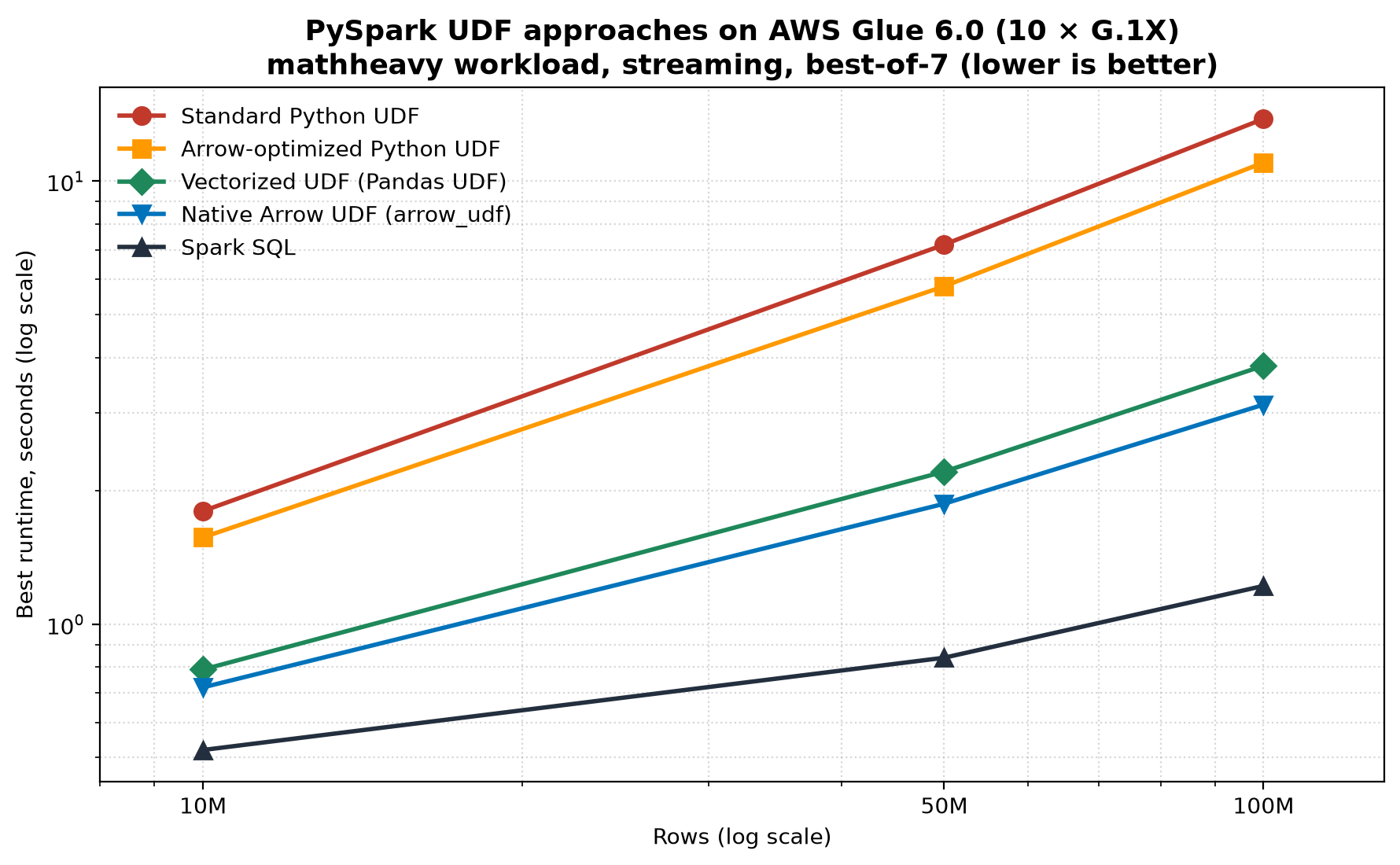
Figure 3: Runtime of each approach on the mathheavy workload across data volumes, on a log-log scale

Workload 3: pyheavy (no SQL equivalent)

This workload runs a per-row iterative loop with no closed-form equivalent. For each row it derives an integer from a and b and repeatedly applies the Collatz step (halve if even, otherwise 3n + 1) until the value reaches 1, counting the number of steps. To keep every row’s runtime predictable, the loop is bounded: it stops after at most 1,000 iterations even if it has not reached 1, so no single row can dominate the benchmark.

def collatz_steps(a, b):             # a, b are scalars (one row per call)
    n = int((a ^ b) % 100000) + 1
    steps = 0
    while n != 1 and steps < 1000:   # bounded: at most 1,000 iterations per row
        n = n // 2 if n % 2 == 0 else 3 * n + 1
        steps += 1
    return steps

This kind of data-dependent control flow can’t be expressed as a SQL scalar expression or with PyArrow compute kernels, so neither Spark SQL nor the native Arrow UDF applies, and only the Python-based UDF approaches are compared. The table shows both query shapes, at 10M, 50M, and 100M rows, to illustrate that the ranking is consistent across shapes and scales:

We report pyheavy up to 100M rows. Because Spark SQL and the native Arrow UDF don’t apply here, the only remaining options are the Python-based UDFs, whose timings scale near-linearly and whose relative order is already stable across both shapes by 100M.

This workload represents the case where a UDF is unavoidable. Examples include an iterative algorithm or a call into a Python library with no SQL counterpart that doesn’t map onto PyArrow compute kernels either. Here the vectorized UDF is the most effective available option: about 2.2× faster than the standard Python UDF at 10M, widening to about 3.8× at 100M.

A controlled experiment: Transport or computation?

The vectorized UDF consistently outperforms the Arrow-optimized Python UDF. To test whether the difference comes from the transport (both use Arrow) or the computation (only the vectorized UDF uses NumPy on a batch), we constructed the missing combination (NumPy computation with pickle transport, no Arrow) using RDD.mapPartitions.

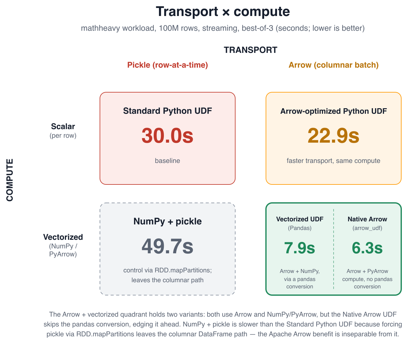
Figure 4: Transport and computation compared as a 2×2 experiment

The NumPy-with-pickle variant was the slowest of all (21.07 seconds at 100M, slower than the standard Python UDF at 13.82 seconds). The reason is that forcing pickle transport requires leaving the DataFrame API for RDD.mapPartitions, which changes two things at once. It materializes each row as a Python object before a NumPy array can be built, and it bypasses the optimized DataFrame execution engine that the vectorized UDF benefits from.

The practical conclusion is that the benefit of a vectorized UDF is not the Arrow transport in isolation. It’s Apache Arrow integrated into the vectorized DataFrame execution path. That path combines columnar transport and NumPy computation. Reproducing only the NumPy portion outside that path doesn’t yield the same benefit.

Code comparison: Arrow-optimized Python UDF and vectorized UDF

These two approaches are often confused: both use Apache Arrow for transport and both show ArrowEvalPython in the physical plan, so it’s worth seeing them side by side. The following two definitions compute the same mathheavy operation. The registration is almost identical. The difference is the function body and the type of its arguments.

The following code is an Arrow-optimized Python UDF (useArrow=True), where the function receives scalar values and runs once per row:

import math
from pyspark.sql.functions import udf
from pyspark.sql.types import DoubleType

def op(a, b):                        # a, b are scalars (one row per call)
    x = float(a % 100000) + 1.0
    y = float(b % 100000) + 1.0
    return math.sqrt(x * x + y * y) * math.sin(x) + math.log(y)

# Arrow transport, scalar Python computation
op_arrow = udf(op, DoubleType(), useArrow=True)
spark.udf.register("op_arrow", op_arrow)

df.selectExpr("sum(op_arrow(a, b)) AS r").collect()

The following code is a vectorized UDF (pandas UDF), where the function receives a pandas.Series (a batch) and computes with NumPy over the whole batch:

import numpy as np
from pyspark.sql.functions import pandas_udf
from pyspark.sql.types import DoubleType

@pandas_udf(DoubleType())
def op_pandas(a, b):                 # a, b are pandas.Series (a batch of rows)
    x = (a % 100000).astype("float64") + 1.0
    y = (b % 100000).astype("float64") + 1.0
    return np.sqrt(x * x + y * y) * np.sin(x) + np.log(y)   # NumPy, whole batch

spark.udf.register("op_pandas", op_pandas)

df.selectExpr("sum(op_pandas(a, b)) AS r").collect()

The following code is a native Arrow UDF (arrow_udf), where the function receives and returns a pyarrow.Array and computes with PyArrow compute kernels, operating directly on Arrow data with no pandas conversion:

import pyarrow as pa
import pyarrow.compute as pc
from pyspark.sql.functions import arrow_udf

@arrow_udf("double")
def op_native(a, b):                 # a, b are pyarrow.Array (a batch of rows)
    x = pc.add(pc.cast(pc.subtract(a, pc.multiply(pc.divide(a, 100000), 100000)), pa.float64()), 1.0)
    y = pc.add(pc.cast(pc.subtract(b, pc.multiply(pc.divide(b, 100000), 100000)), pa.float64()), 1.0)
    return pc.add(pc.multiply(pc.sqrt(pc.add(pc.multiply(x, x), pc.multiply(y, y))), pc.sin(x)), pc.ln(y))

spark.udf.register("op_native", op_native)

df.selectExpr("sum(op_native(a, b)) AS r").collect()

The Arrow-optimized Python UDF and the vectorized UDF differ in two lines that matter:

• Argument type – In the Arrow-optimized UDF, a and b are scalars, so the body uses math.sqrt and math.sin and runs once per row. In the vectorized UDF, a and b are pandas.Series, so the body uses np.sqrt and np.sin and runs once per batch.
• Where the computation runs – The Arrow-optimized UDF still executes Python per row. The vectorized UDF executes the batch in NumPy’s native code.

This difference in where the computation runs is what separates the three at scale. On the mathheavy workload at 100 million rows, the Arrow-optimized UDF ran in 11.01 seconds, the vectorized UDF in 3.83 seconds, and the native Arrow UDF fastest at 3.13 seconds. The native Arrow UDF edges ahead because it vectorizes the computation through PyArrow compute kernels without the pandas conversion the vectorized UDF performs. However, it requires the logic to be expressible with those kernels, where the vectorized UDF remains the more flexible choice.

Recommendations

These results align with the AWS Prescriptive Guidance recommendation and add a few practical points:

1. Prefer built-in Spark SQL functions when the operation can be expressed in SQL – The computation runs on the JVM, and the advantage grows with data volume.
2. When a UDF is required and the logic can be expressed with PyArrow compute kernels, consider a native Arrow UDF (arrow_udf) – In our tests it was the fastest UDF approach, because it vectorizes the computation on Arrow data without a pandas conversion. It’s available in AWS Glue 6.0 (Apache Spark 4.1).
3. Otherwise, use a vectorized UDF (pandas UDF) – It outperformed the standard Python UDF by 2.2–3.8× in our tests. It’s the more flexible option when the logic is easier to express with pandas or NumPy than with PyArrow compute kernels.
4. Arrow-optimized Python UDFs (useArrow=True) improve the transport but not the computation – They are faster than the standard Python UDF, but a vectorized or native Arrow UDF is faster whenever the per-row work is non-trivial. Consider the Arrow-optimized Python UDF when you want a minimal change to an existing scalar UDF.
5. Stay in the DataFrame API to keep Arrow’s benefit – As the controlled experiment showed, the speedup doesn’t come from Arrow serialization alone. It comes from Arrow integrated into the vectorized DataFrame execution path. Applying the same NumPy logic through RDD.mapPartitions was the slowest approach of all, because it leaves that path. Implement vectorized logic as a vectorized or native Arrow UDF within the DataFrame API rather than dropping to the RDD API.
6. For iterative or data-dependent logic (the pyheavy case), the vectorized UDF is the fallback – When the operation maps onto neither SQL nor PyArrow compute kernels, both Spark SQL and the native Arrow UDF are unavailable, and among the remaining Python UDF approaches the vectorized UDF was the most efficient.
7. Decide whether the rewrite is worth the effort – Moving a scalar UDF to a vectorized or native Arrow UDF is a small code change, but it still has to be written and tested. As a rule of thumb, it pays off when the per-row work is non-trivial and the data is large or the job runs often. The speedup (and the per-second cost saving) scales with row count and with how frequently the job runs, while the rewrite is a one-time cost. For a trivial operation on a small, infrequent dataset, the standard Python UDF might be perfectly adequate. For a compute-heavy transform on hundreds of millions of rows that runs daily, the rewrite typically repays itself in the first few runs.
8. The exact numbers depend on your cluster – All results here use a fixed configuration (10 × G.1X workers) on AWS Glue 6.0. The ranking of approaches is a property of how each UDF crosses the JVM–Python boundary and is not expected to change with cluster size. However, the absolute timings and any crossover with alternatives will shift with worker count, worker type, and data layout. Treat the figures as a guide to relative behavior and validate against your own configuration.
9. Methodology affects the outcome – Warm-up handling and cache management changed our ranking. A UDF benchmark whose timings don’t scale with row count is likely measuring the cache.

Conclusion

The choice of UDF strategy has a measurable and recurring impact on both runtime and cost. On our compute-intensive workload at 100 million rows, the gap between the fastest UDF approach (the native Arrow UDF at 3.13 seconds) and the standard Python UDF (13.82 seconds) was about 4.4×, for identical output. Because AWS Glue bills by the second, that difference translates directly into spend on every job run.

These results extend the AWS Prescriptive Guidance recommendation with volume scaling from 10 million to 100 million rows, a compute-intensive workload, and the newer Arrow-based UDF options available in AWS Glue 6.0 (Apache Spark 4.1). As a methodology note, warm-up handling and cache management materially affected the ranking. A UDF benchmark whose timings don’t scale with row count is likely measuring the cache rather than the computation.

To learn more, see Optimize user-defined functions in AWS Prescriptive Guidance and the AWS Glue documentation.

About the author