AWS Big Data Blog
Querying raw log data using SQL and PPL with the optimized engine in Amazon OpenSearch Service
In this post, you learn how to run fast analytical queries directly against raw log and trace data in Amazon OpenSearch Service using PPL and SQL.
Amazon OpenSearch Service is a fully managed service that helps you deploy, scale, and operate OpenSearch, the open source suite for search, analytics, and observability in the AWS Cloud. OpenSearch Service powers search and real-time analytics workloads, from lexical and hybrid search to log analytics and observability. This post focuses on log analytics, and on a practical question: how much analytical work can you do directly against raw log and trace data, without moving it or reshaping it first?
The new optimized engine in OpenSearch Service answers that question: you can point Piped Processing Language (PPL) and Structured Query Language (SQL) queries at raw log and trace data. The engine returns aggregations, filters, and scans over billions of events on the data exactly as you ingested it. In this post, you follow a single incident investigation, one query at a time. You see how the engine answers each new question, from multi-dimensional breakdowns and latency distributions to error rates and fleet sizing. No precomputed structure sits behind the results.
How the optimized engine queries raw data
The optimized engine stores data in the columnar Apache Parquet format and runs queries through Apache DataFusion, a vectorized execution engine, with Apache Calcite planning each query. Because the engine stores data in columns, an analytical query reads only the columns it touches and processes their values in batches, instead of reading each matching document in full. Alongside the columnar format, the engine also keeps an inverted index on the same data, so the query planner routes each operation to the path that serves it best: the columnar engine for aggregations and analytical scans, and the inverted index for selective search and filtering.
You ingest your logs and traces through the same Bulk API and clients you use today, and you write PPL or SQL against them as they land.
An investigation, one query at a time
The following walkthrough traces a common observability use case, root-cause analysis during a live incident, from the perspective of a site reliability engineer (SRE). The engineer notices elevated latency and a handful of error alerts, with nothing that points to a clear cause. No existing dashboard covers this particular shape of problem, so the engineer opens Amazon OpenSearch Service and starts asking questions of the raw trace data, letting each answer decide the next one. PPL suits this work well. Each command transforms the data and passes it to the next, so the engineer reads a query left to right the same way they think through the investigation.
The walkthrough uses generated OpenTelemetry (OTEL) data from a synthetic load generator, at billion-document scale. The focus is the query capability, that is, what the engineer can express and retrieve directly from raw spans, rather than the specific values in each result.
Step 1: Assess the scope
The first question in any investigation is how widespread the signal is. The engineer breaks errors down across service, HTTP method, and cloud Region in a single pass over roughly 1.1 billion spans.
In plain terms, this query answers the engineer’s first question: where are the failures happening? It counts the error spans and breaks them down by service, HTTP method, and AWS Region in a single pass. Rather than guessing which service to open first, the engineer gets a ranked list of the hardest-hit combinations to investigate.
| errors | total_count | avg_ns | serviceName | http_method | cloud_region |
| 730 | 112,436 | 41,246,806 | export-service | GET | us-west-2 |
| 722 | 111,215 | 41,000,227 | catalog-service | PUT | eu-central-1 |
| 704 | 112,051 | 41,295,539 | image-service | PATCH | us-west-2 |
| 612 | 93,214 | 41,451,145 | healthcheck-service | PUT | us-east-1 |
| 609 | 94,314 | 41,418,897 | auth-service | POST | us-east-1 |
| 609 | 94,414 | 41,447,444 | email-service | PATCH | ap-northeast-1 |
| 593 | 89,726 | 41,047,114 | payment-service | PUT | eu-central-1 |
| 581 | 89,854 | 41,195,643 | file-service | PUT | ap-northeast-1 |
The errors spread across services, methods, and Regions, which points to a systemic pattern rather than a single misbehaving service.
Step 2: Check whether one host concentrates the failures
The spread could still reflect one saturated node or a fleet-wide condition. To tell the two apart, the engineer groups failures by exception type, service, and host across the entire index, with no time filter to narrow the scan.
| total_count | exception_type | serviceName | host_name |
| 6 | DeadlockDetectedException | notification-service | ip-10-0-16-34 |
| 6 | IllegalStateException | api-gateway | ip-10-0-180-234 |
| 6 | FileNotFoundException | cart-service | ip-10-0-90-162 |
| 6 | ConnectionRefusedException | feature-flag-service | ip-10-0-8-123 |
| 5 | TimeoutException | auth-service | ip-10-0-97-78 |
| 5 | ConcurrentModificationException | order-service | ip-10-0-165-15 |
| 5 | TimeoutException | coupon-service | ip-10-0-158-25 |
In this sample the counts are low and every row lands on a different host, so no single node stands out. This points to a fleet-wide pattern rather than one bad machine. On production data the same query makes the distinction directly: a code-level bug shows up across many hosts, whereas a single failing node concentrates its errors on one host_name.
Step 3: Quantify the latency distribution per service
Next, the engineer pulls a latency profile for each service. This includes count, average, minimum, and maximum duration, to see how each one behaves and how wide the spread runs.
| serviceName | total_count | avg (ns) | min (ns) | max (ns) |
| event-bus | 11,087,263 | 41,249,552 | 26,113 | 9,304,132,159 |
| scheduler-service | 9,175,964 | 41,251,927 | 21,919 | 13,432,040,933 |
| cdn-service | 9,173,572 | 41,225,385 | 23,468 | 13,768,293,306 |
| ml-inference | 9,036,753 | 41,289,101 | 40,410 | 14,625,084,517 |
| compliance-service | 8,274,635 | 41,294,694 | 41,915 | 7,462,983,016 |
| metrics-collector | 7,804,234 | 41,334,728 | 16,535 | 23,228,217,669 |
| notification-service | 7,688,714 | 41,204,635 | 51,562 | 8,695,311,374 |
| image-service | 7,674,406 | 41,248,069 | 47,473 | 15,350,500,299 |
This gives the engineer a latency fingerprint for each service: the averages sit near 41 milliseconds. But the multi-second maxima reveal a long tail consistent with requests queuing behind a slow dependency.
Step 4: Measure the error rate per service
To track a service-level objective, the engineer computes the error rate (errors against total requests) per service. The query uses an inline conditional, followed by a grouped sum and count, and a final division to produce the error rate.
| errors | total_count | error_pct | serviceName |
| 699,358 | 22,415,308 | 3.12 | payment-service |
| 647,811 | 26,880,140 | 2.41 | checkout-service |
| 562,811 | 30,096,860 | 1.87 | auth-service |
| 316,192 | 24,510,990 | 1.29 | cart-service |
| 288,314 | 30,671,704 | 0.94 | order-service |
| 202,612 | 28,140,552 | 0.72 | search-service |
| 186,012 | 33,820,415 | 0.55 | catalog-service |
| 134,722 | 35,453,247 | 0.38 | image-service |
The engineer defines the error-rate metric in the query itself, and the engine computes it across the full index. The busiest paths, payment and checkout, run near 3 percent, whereas some services stay below 1 percent.
Step 5: Size the fleet footprint with SQL
Finally, the engineer sizes how much of the fleet each service spans, a capacity and impact question, and switches from PPL to SQL to express it.
| serviceName | total_count | hosts |
| ml-inference | 35,481,688 | 2,535 |
| image-service | 35,453,247 | 2,491 |
| email-service | 35,443,569 | 2,517 |
| shipping-service | 30,700,372 | 2,438 |
| translation-service | 30,490,570 | 2,502 |
| auth-service | 30,096,860 | 2,466 |
| chat-service | 25,564,111 | 2,449 |
| recommendation-service | 25,366,844 | 2,483 |
The query runs a COUNT(DISTINCT) over a high-cardinality field at billion-row scale, and switching languages mid-investigation costs the engineer nothing more than writing SQL instead of PPL. The host counts cluster in the approximately 2,400–2,540 range, so each service runs across a broad slice of the fleet. That confirms the earlier finding: the errors reflect a fleet-wide pattern, not a single node.
The engineer asked five questions and ran five queries, and each answer shaped the next. The optimized engine served every query directly from raw trace data, across both PPL and SQL, without a rollup table or precomputed summary behind any result.
Run these queries where you already work
You don’t need a separate tool to run the queries in this walkthrough.
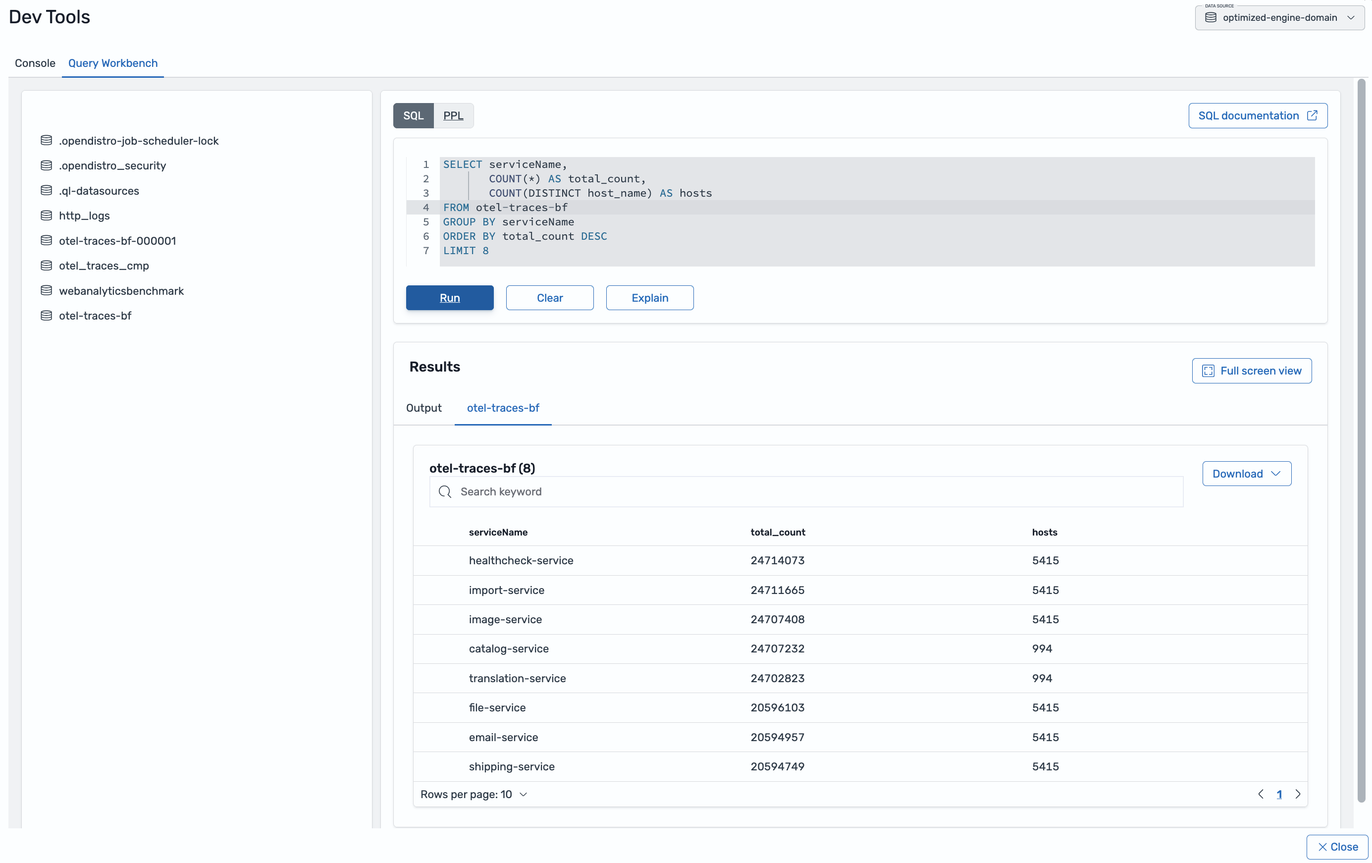
Figure 1: Investigation queries and results grid in Query Workbench
Query Workbench in OpenSearch Dashboards UI gives you a dedicated editor for PPL and SQL. You write a query, run it, and read the results in a grid, using the same queries shown throughout this post. When you want to move from a written query to interactive exploration, Discover runs the same PPL and SQL against your indexes. In Discover, you can filter, expand fields, and drill into individual documents without leaving the page. The same query language works in both places, so you can start an investigation in Discover and carry it into Query Workbench, or the reverse, without rewriting anything.
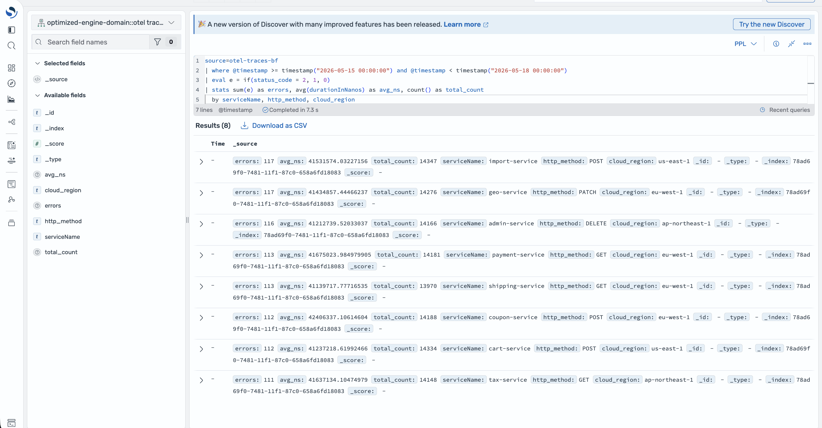
Figure 2: PPL query and field list in Discover
Keep all your data and query it as it is
Querying raw data directly only helps if you can afford to keep the raw data. The optimized engine compresses observability data up to 70 percent more efficiently than the default General Purpose engine. That compression turns “keep everything and query it directly” into a practical default. You retain full-fidelity data for the questions you cannot predict in advance. You also pay less to store it than you would to store the raw JSON.
Get started
To try the optimized engine, create an Amazon OpenSearch Service domain running OpenSearch 3.5 or later. Then select the Observability use case during setup, which provisions the domain with the optimized engine.
To learn more about configuring and using the optimized engine, see Optimized for Log Analytics in the Amazon OpenSearch Service documentation. For an overview of the service, visit Amazon OpenSearch Service Log Analytics.
For more information, see the blog post Run log analytics for a fraction of the cost with the new engine for Amazon OpenSearch Service.
Give it a try and send feedback to AWS re:Post for Amazon OpenSearch Service or through your usual AWS Support contacts.