AWS Storage Blog
Scaling a Weaviate vector index 26× with one Amazon EBS gp3 command
We thought high-performance vector databases were memory bound. Then we raised a single Amazon Elastic Block Store (Amazon EBS) gp3 volume from its 3,000 IOPS default to its 80,000 IOPS maximum. The same node (a c6in.8xlarge with 64 GiB RAM, running Weaviate’s disk-based HFresh vector index in a container capped at 8 GiB) went from 9.8 to 260 queries per second (QPS) on the same 10-million-vector index. Nothing else changed. We used a large instance size deliberately: its EBS-optimized throughput is sustained, not burst-limited. A true 8-GiB-RAM instance such as a c6in.xlarge can reach these IOPS only during its approximately 30-minute daily burst window before dropping to a lower baseline, so it would not hold these numbers.
Vector search has been described as a RAM problem for a decade now. The Hierarchical Navigable Small World (HNSW) index that most vector databases use keeps every vector and graph edge in memory, so capacity planning starts with “how many gigabytes of vectors do we have” and ends with a large instance and increased costs. Weaviate’s HFresh index, generally available since Weaviate 1.38, changes that: it keeps a small centroid index in memory and reads everything else from disk. That makes storage I/O the deciding factor in query performance, and Amazon EBS gp3 puts that factor under your control with a single API call.
This post shows how HFresh reads the disk, measures the impact that gp3 and Elastic Volumes modifications have on query throughput on one node, and demonstrates how EBS takes a Weaviate cluster from “startup” to “enterprise” search scale with a single CLI command.
Why HFresh reads the disk the way it does
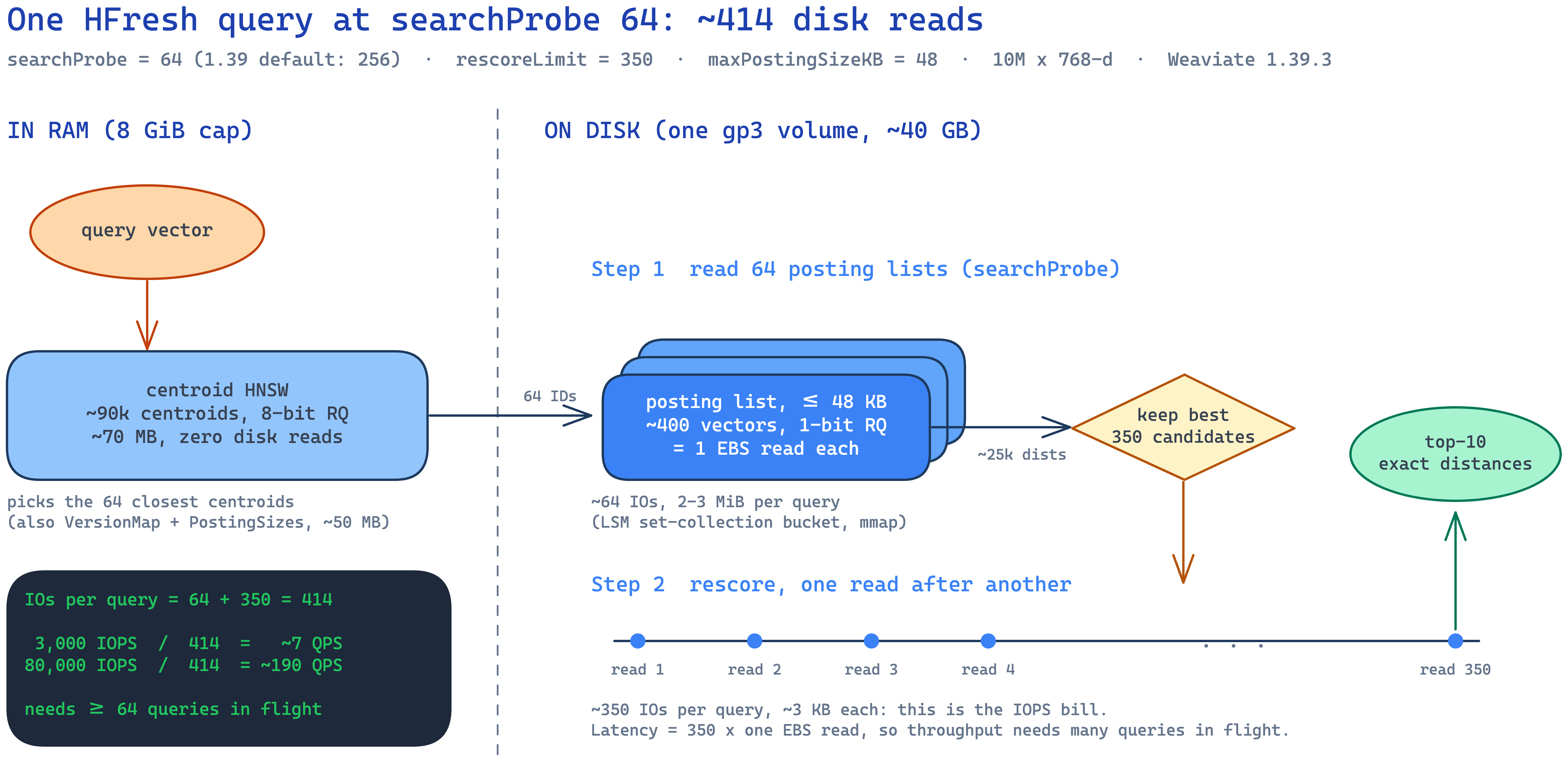
Figure 1: The read path of one HFresh query at the settings used in this post
Weaviate’s HFresh index, inspired by the SPFresh algorithm, divides vectors into small clusters called postings. Each posting holds a few hundred vectors compressed to 1 bit per dimension with rotational quantization and is stored as one record, at most 48 KB, in Weaviate’s LSM store on disk. The centroids of those postings live in a small in-memory HNSW graph (8-bit quantized, about 70 MB for the index in this post).
A query does three things:
- Searches the in-memory centroid graph to pick the closest
searchProbepostings. No disk access. - Reads those postings from disk and scores every vector in them with the 1-bit representation. One read per posting.
- Rescores the best
rescoreLimitcandidates against their full-precision vectors, which live in the object store on disk. One small random read per candidate, issued one after another.
At searchProbe 64 and rescoreLimit 350 that is roughly 414 disk reads per query, dominated by step 3. Two consequences follow. First, throughput is a function of the IOPS the volume delivers. Second, because the rescoring reads are serial within a query, a single query’s latency is about 350 times one disk read, so throughput only comes from running many queries concurrently. Both knobs are mutable at runtime, which let us vary them without re-indexing.
The Amazon EBS gp3 performance envelope
At Weaviate we host all of our AWS customers on EBS gp3 volumes. Every gp3 volume comes with 3,000 IOPS and 125 MiB/s at no extra charge, at any size, and we frequently increase the limits for customers with heavy usage. Since September 2025 a single gp3 volume can be provisioned up to 80,000 IOPS and 2,000 MiB/s, five times the previous IOPS ceiling, which we use to deliver high performance for Weaviate.
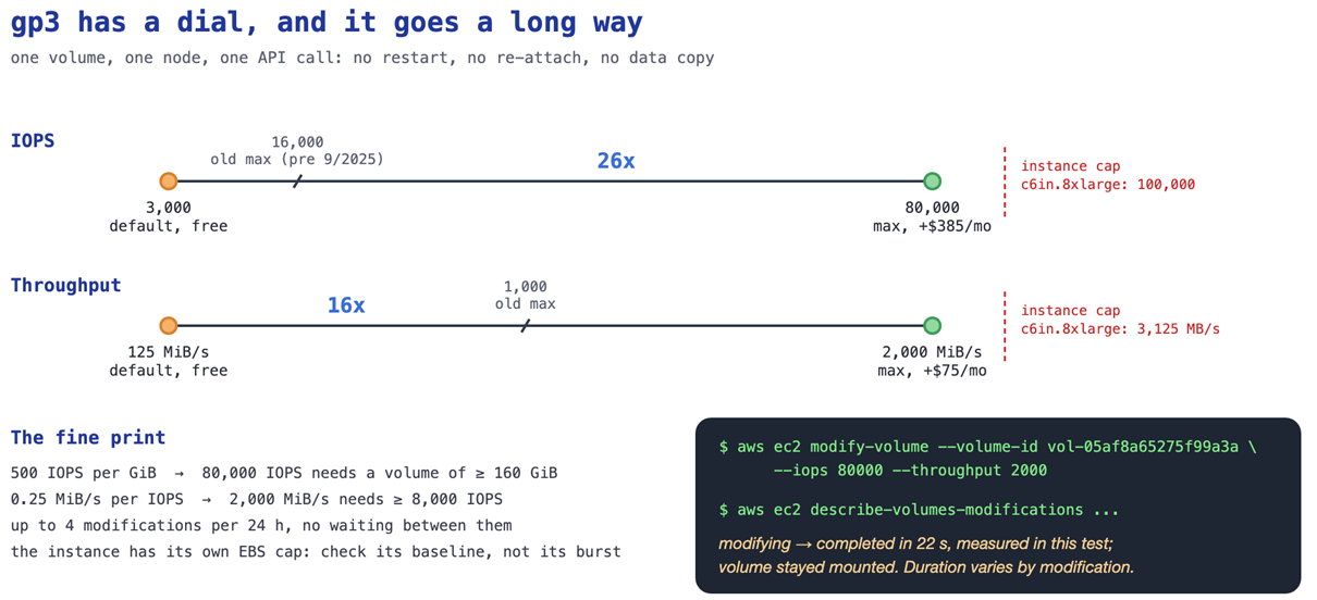
Figure 2: What one gp3 volume can be provisioned to, and the rules that apply
Benchmark test overview
We ran the benchmark in four steps:
- Import once at the maximum setting. Ingesting 10 million vectors and letting HFresh’s background split, merge and reassign work finish took about 20 minutes at 80,000 IOPS, with the container temporarily allowed 32 GiB. The bytes on disk are the same regardless of how fast they were written, so the import setting has no bearing on the query results.
- Reset before every phase. Stop the container, drop the page cache, pin
read_ahead_kbto 16 (the 128 KB default turns a 3 KB rescoring read into a 128 KB read and makes the volume look throughput-bound), start the container under the 8 GiB cap, run a discarded 60-second warm-up. - Run the same tests at each volume setting. Concurrent clients 8, 32 and 128, times
searchProbe32, 64, 128 and 256, thenrescoreLimitvalues of 100, 350 and 1,000 at 32 clients. - Capture the host.
iostat -xevery second, the container’s cgroupmemory.currentevery 5 seconds, and Weaviate’s Prometheus metrics every 10 seconds, so every QPS figure has the disk and memory picture beside it.
We ran the maximum setting first, then modified the volume down to the default and ran the baseline. We present the results in the natural order.
Benchmarking system configuration
Here is the configuration we used to test it:
| Component | Configuration |
| Server instance | c6in.8xlarge (32 vCPU, 64 GiB), Amazon Linux 2023 |
| Weaviate | 1.39.3, single node, in a container with a hard 8 GiB cgroup memory limit (page cache included), no swap, GOMEMLIMIT 5 GiB, GOMAXPROCS 24 |
| Data volume | One gp3, 400 GiB, encrypted, ext4 with noatime, read_ahead_kb pinned to 16 |
| Dataset | sphere-10M-meta-dpr from the Weaviate ANN benchmark set: 9,990,000 vectors, 768 dimensions. |
| Vector index | HFresh, maxPostingSizeKB 48, replicas 4, rq.rescoreLimit 350, searchProbe tested at 32, 64, 128 and 256 (256 is the 1.39 default) |
| On-disk footprint after import | 39 GB, almost five times the memory cap |
| Load generator | weaviate-benchmarking (benchmarker ann-benchmark) over gRPC, k = 10, on a separate c7i.2xlarge in the same Availability Zone |
| Infrastructure | Terraform. Access through an EC2 Instance Connect Endpoint, no public ingress |
Before every phase we calibrated the volume with the standard open-source disk testing application fio (4 KiB random reads, queue depth 256) to prove that it delivered what was provisioned:
| Volume setting | Measured random-read IOPS | Measured sequential MiB/s |
| 3,000 IOPS / 125 MiB/s | 3,049 | 129 |
| 80,000 IOPS / 2,000 MiB/s | 81,389 | 2,100 |
Benchmark test results
Part 1: The gp3 default, 3,000 IOPS / 125 MiB/s
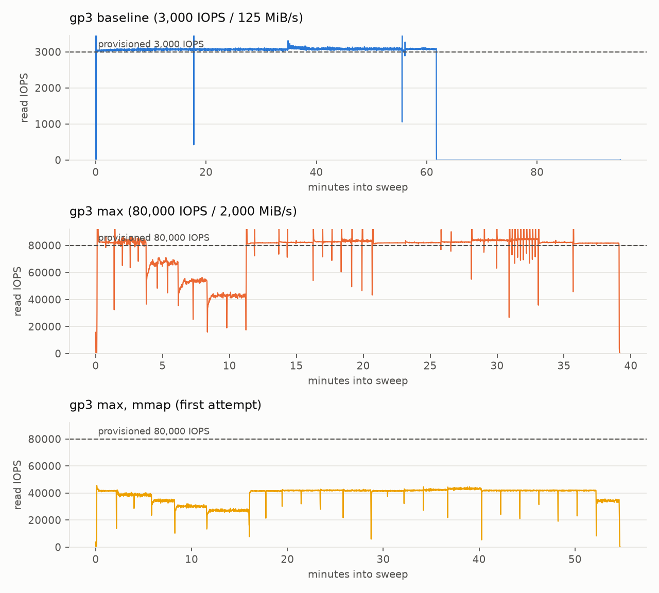
Figure 3: Read IOPS delivered by the volume during each test run. Top: the default setting, pinned at its 3,000 IOPS ceiling for the whole hour. Middle: the maximum setting. Bottom: the maximum setting with Weaviate’s default mmap access strategy (Part 4)
| Clients | searchProbe | QPS | Mean latency | p99 latency |
| 8 | 32 | 10.2 | 784 ms | 1,284 ms |
| 8 | 64 | 9.8 | 817 ms | 1,426 ms |
| 8 | 128 | 9.1 | 871 ms | 1,710 ms |
| 8 | 256 | 8.5 | 933 ms | 1,992 ms |
| 32 | 64 | 9.8 | 3,248 ms | 5,708 ms |
| 32 | 256 | 8.1 | 3,927 ms | 8,726 ms |
The volume sat at 3,074 read IOPS on average, 100 percent utilized, with a mean read wait of 64 ms and about 200 reads queued. Reads averaged 9.2 KiB, so throughput was 28 MiB/s against a 125 MiB/s allowance: the IOPS limit, not the throughput limit, was binding, as predicted. Going from 8 to 32 clients changed nothing but latency. Host CPU was mostly idle. Nothing about this node was busy except the disk queue.
At 9.8 QPS and 3,074 IOPS the node spent about 314 reads per query, close to the 414 estimate (some posting reads hit the page cache).
Part 2: Live volume modification with one command
This is why we love EBS: one command changes the performance of a live volume. We ran the following command to change the performance profile of the volume:
No detach or restart is necessary. You can run this command on a live volume, and we ran it with the volume mounted and Weaviate running. In our run, raising the volume from the default to the maximum reached optimizing in about 22 seconds with the new IOPS and throughput usable almost immediately. modify-volume is best-effort, and how long a modification takes varies from change to change. The practical takeaway is that the usable performance change and the optimizing completion are decoupled in both directions. You do not need to block on the completed state if you script modifications. Act on the applied performance, verified with fio or the describe-volumes-modifications progress, rather than waiting for optimizing to finish.
Part 3: The gp3 maximum, 80,000 IOPS / 2,000 MiB/s
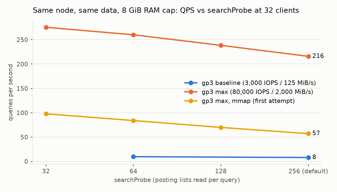
Figure 4: Queries per second at 32 concurrent clients as searchProbe grows, same node, same data, same 8 GiB cap
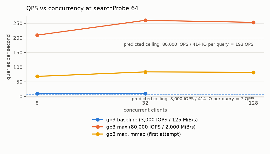
Figure 5: Queries per second against concurrent clients at searchProbe 64, with the predicted IOPS ceilings
| Clients | searchProbe | QPS | Mean latency | p99 latency |
| 8 | 32 | 279.5 | 28 ms | 45 ms |
| 8 | 64 | 209.5 | 38 ms | 60 ms |
| 8 | 128 | 153.6 | 52 ms | 87 ms |
| 8 | 256 | 115.4 | 69 ms | 127 ms |
| 32 | 32 | 275.5 | 115 ms | 176 ms |
| 32 | 64 | 260.1 | 122 ms | 204 ms |
| 32 | 128 | 238.4 | 132 ms | 235 ms |
| 32 | 256 | 215.9 | 145 ms | 269 ms |
| 128 | 32 | 270.5 | 465 ms | 764 ms |
| 128 | 64 | 253.2 | 494 ms | 808 ms |
| 128 | 128 | 219.7 | 570 ms | 985 ms |
| 128 | 256 | 178.0 | 704 ms | 1,236 ms |
With 32 concurrent clients and searchProbe 64, the node delivered 260 QPS, 26.5 times the default setting’s 9.8 QPS. The p99 latency fell from 5.7 seconds to 204 ms, a 28-fold reduction. The volume averaged 76,806 read IOPS across the test run, 25 times the baseline, with reads still averaging 9.3 KiB for a throughput of 700 MiB/s against the 2,000 MiB/s allowance. QPS scaled with IOPS almost one for one, which is what a disk-bound system looks like. A traditional in-memory HNSW index would need roughly seven times the memory used here: by Weaviate’s own rule of thumb of twice the raw vector size, these 10 million 768-dimension vectors need about 61 GB uncompressed, compared with the 8 GiB cap.
Recall was identical at both settings for every searchProbe value, because the index and the data were identical. The absolute recall figures are low for a reason unrelated to storage: this dataset’s ground truth is computed with the dot product on vectors that are not unit length (mean norm 14.4), while HFresh supports cosine and L2 only. Treat recall here as a consistency check between phases, not as HFresh’s recall.
Part 4: The default access strategy capped the volume at half its IOPS
With the default mmap access strategy, our first test run at the maximum setting reached only 39,000 read IOPS and 82 QPS regardless of client count: 32 clients and 128 clients produced the same throughput, with the extra clients only adding latency. Host CPU showed 68 percent iowait and 2 percent user time. The volume had 25 reads in flight when it needed well over 150.
| Access strategy | Reads in flight (iostat aqu-sz, median) | Read IOPS | QPS at 32 clients, searchProbe 64 |
mmap (Weaviate default) |
25 | 38,860 | 84.0 |
pread |
167 | 76,806 | 260.1 |
The explanation is in the read path. With Weaviate’s default mmap access strategy every posting or object read that misses the page cache is a page fault. A page fault pins the operating-system thread that took it until the read completes. The Go runtime had GOMAXPROCS set to 24 with Go 1.26. So at most about two dozen reads could be outstanding at any moment. A gp3 volume only delivers 80,000 IOPS with a few hundred outstanding at 2 to 3 ms each. Setting PERSISTENCE_LSM_ACCESS_STRATEGY=pread turns those reads into ordinary system calls that the runtime hands off, and the same volume went to 77,000 IOPS and three times the QPS. Every number in Parts 1 and 3 uses pread. If you run a disk-backed vector index on a high-IOPS volume, this setting is the first thing to check.
Part 5: The memory cap held
To confirm that the volume, not the page cache, was serving the queries, we tracked the container’s memory throughout both test runs.
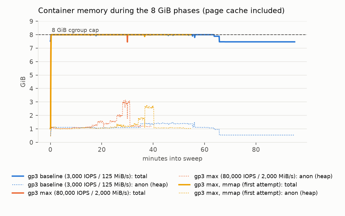
Figure 6: Container memory (cgroup memory.current) during both 8 GiB test runs, with the anonymous (Go heap) portion dotted
In every run the container sat at exactly 8.00 GiB: between 1.5 and 3.1 GiB of heap and the rest page cache, against 39 GB on disk. Nothing was cached away. The disk really was serving the queries, and the only thing that changed between 9.8 and 260 QPS was the volume’s provisioned performance.
Cost and performance
Monthly prices are US East (Ohio) on-demand, 730 hours, at the time of the test.
| Configuration | Instance | Volume | Provisioned IOPS and throughput | Total per month | QPS (32 clients, probe 64) | Per 100 QPS per month |
| c6in.8xlarge, 8 GiB cap, gp3 default | $1,324 | $32 | $0 | $1,356 | 9.8 | $13,840 |
| c6in.8xlarge, 8 GiB cap, gp3 maximum | $1,324 | $32 | $460 | $1,816 | 260 | $698 |
The IOPS and throughput uplift added 34 percent to the monthly bill and 26.5 times the throughput, a 20-fold improvement in cost per query. The Amazon Elastic Compute Cloud (Amazon EC2) instance dominates the bill and was chosen for its 100,000 IOPS EBS limit, not its CPU or memory (most of which sat idle). Customers with bursty I/O can often cut compute cost further by downsizing to a smaller instance that supports EBS-optimized burst, which lets short spikes exceed baseline. Keep in mind that burst is a credit budget (approximately 30 minutes/day at the ceiling). Size for your sustained I/O and burst duration, not the peak.
Recommendations
These recommendations come from this test. They apply to teams running a disk-backed vector index such as Weaviate’s HFresh on Amazon EBS gp3, and the volume and instance sizing points apply to most read-heavy workloads on gp3:
- Set PERSISTENCE_LSM_ACCESS_STRATEGY=pread for any disk-backed Weaviate index on a volume provisioned above the default. With
mmap, in-flight reads are capped nearGOMAXPROCSand the volume will not reach its IOPS. - Size the volume for the IOPS, not the data. 80,000 IOPS requires at least 160 GiB. 2,000 MiB/s requires at least 8,000 IOPS.
- Check the instance’s EBS limit first. It is often lower than the volume’s maximum.
- Pin readahead small on the data volume. Fault-around and readahead inflate small random reads and shift the bottleneck from IOPS to throughput without adding useful work.
- Tune rescoreLimit before adding IOPS. It sets the reads per query.
searchProbesets recall. Both are runtime settings. - Modification time depends on what you change, not on direction. Size increases reach optimizing in seconds and are usable immediately (size can only grow, so a true “scale-down” of capacity is not supported). IOPS/throughput changes, up or down, take minutes to hours, roughly 6 hours for a fully used 1-TiB volume, longer if larger or not fully initialized. Plan scripted scale-downs around this: you can modify a volume at most 4 times in a rolling 24-hour period, and each modification must reach completed before the next. Note billing starts at the new configuration as soon as the modification begins, and provisioned IOPS/throughput bill regardless of attachment.
- This is one node, one dataset, one distance metric and one volume. Striping several gp3 volumes, io2 Block Express and instance-store NVMe were not tested. Serial rescoring is an implementation detail of the current HFresh and might change.
Conclusion
A disk-backed vector index replaces fixed memory requirements with tunable storage performance, and with Amazon EBS gp3 you can tune it with a single API call on a live volume. On one c6in.8xlarge with Weaviate capped at 8 GiB, raising a gp3 volume from 3,000 to 80,000 IOPS took a 10-million-vector index from 9.8 to 260 queries per second with p99 latency down from 5.7 seconds to 204 ms, for 34 percent more per month. The point is not that disk beats RAM per query. It is that the disk tier now has a dial, and the dial goes a long way.
To learn more, see the Amazon EBS User Guide on gp3 volumes and the Weaviate documentation on the HFresh vector index. If you have questions or comments, leave them in the comments section.
To reproduce these benchmarks, visit the Weaviate GitHub repository, which contains the Terraform, the container definition, the test and capture scripts, the raw results and the chart renderer. Import takes about 20 minutes at the maximum setting, and each test run takes 40 minutes at the maximum setting and about an hour at the default.
FAQ
Why use gp3 and not io2?
gp3 is the lowest-cost SSD volume type in Amazon EBS and the default when you create a volume in the Amazon EC2 console, and AWS recommends General Purpose SSD volumes for most workloads. Its performance can be changed on a live volume for a marginal cost. The question we wanted to answer was what the default dial does. io2 reaches 256,000 IOPS and sub-millisecond latency and is the obvious next test.
Will striping multiple gp3 volumes increase performance?
Yes, up to the instance’s EBS limit. A single volume was used so that one ModifyVolume call would be the only variable.
Does this apply to HNSW?
No. HNSW keeps vectors and graph in memory and does not read the volume during a query. The result is specific to disk-backed indexes such as HFresh.
Does gp3 provisioning also speed up writes?
This test measured query performance only. The initial import of 10 million vectors ran at 80,000 IOPS and finished in about 20 minutes, but we did not measure how write throughput changes with the volume settings. HFresh is designed for continuously changing data, so a write-heavy test is a topic for a separate post.
Why is recall@10 around 0.5?
Recall@10 is the fraction of each query’s 10 true nearest neighbors that the search returns, so 0.5 means about half of them. It is low here because the dataset’s ground truth uses the dot product on non-unit vectors and HFresh supports cosine and L2 only. Recall was identical at both volume settings, which is the property this test needed.