AWS Database Blog
Amazon Aurora under the hood: indexing geospatial data using Z-order curves
When designing high-performance database systems like Amazon Aurora, you typically want to work on things that deliver the most impact for the broadest set of workloads. But sometimes, it pays to focus on specialized use cases where you have the opportunity to change the game.
In this post, let’s take a look at how Aurora has changed the game for geospatial workloads. Most OLTP systems perform poorly for geospatial workloads, limiting their effectiveness. Aurora uses z-order curves for geospatial indexing to deliver performance improvement an order of magnitude over MySQL R-trees. These improvements make it feasible to operate high-throughput OLTP workloads over geospatial data.
What is geospatial indexing, and why do I care?
Geospatial analysis allows you to identify nearness, adjacency, and overlap along XY(Z) coordinates.
There are obvious examples of applications that need to be able to perform such analyses. A ride hailing app should allow customers to find the nearest available cab. A real estate app should be able to show the properties are listed for sale within the Pacific Heights district in San Francisco.
It turns out that spatial analysis can also be valuable in a number of other domains, such as these and similar ones:
- Marketing—target a promotion to all prospects within two miles of store.
- Asset management—locate repair units to minimize impact based on customer location and density.
- Risk analysis—estimate risk premiums based on incidence of car thefts in locations next to the customer’s residence and workplace.
- Fraud detection—estimate likelihood of a fraudulent transaction based on distance from previous transaction.
- Logistics planning—assign trouble tickets to field technicians to minimize radius of travel.
These applications can obviously benefit from a high-performance index on the underlying spatial data. Unfortunately, traditional indexes like B-trees were built for Lineland, not so much for Flatland or Spaceland ;). Thus, there’s a need for a high-performance geospatial index.
What about R-trees?
The most commonly used spatial index is the R-tree (for more about this, see this paper by Guttman84). Both MySQL and Oracle use R-tree. The basic idea is to store bounding rectangles in a balanced search tree. The leaves are data points, and each interior node is the minimum bounding rectangle for the nodes under it. So, in the example following, rectangle A is a leaf node. This node is bounded in turn by rectangles N and T.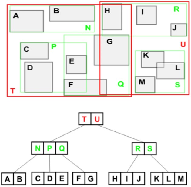
The main issue with R-trees is that they are not stable (that is, deterministic). Different insertion orders result in different trees, with very different performance characteristics. In our tests, we found that a random insertion order produced a tree that performed an order of magnitude worse than a tree built in the optimal order. This is clearly a problem in OLTP environments, where the data comes in an unpredictable order and is mutable. In such a situation, R-trees degenerate over time. One workaround is to periodically reindex the data. However, the reindexing operation is expensive. It typically requires manual effort, can take hours, and slows down other transactions during that period.
That’s why R-trees, although popular, don’t deliver a ton of performance.
Is there a better way?
We think so! There’s a data structure that’s great for transactions and concurrency. It’s a B-tree. It’s foundational to databases, used everywhere, and highly performant.
But, hold on a minute. Didn’t I just say B-trees don’t work well for multi-dimensional data? Well, that’s true. The trick to map 2D space into 1D.
We do this using space-filling z-order curves. Briefly, the z-value of a point is calculated by interleaving the binary representations of its coordinate values. The z-order curve is the line that traverses these points in order of z value. For example, the figure following shows the z values for the case with integer coordinates 0 ≤ x ≤ 7, 0 ≤ y ≤ 7 (shown both in decimal and binary).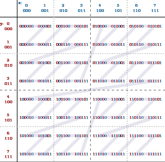
A simple implementation of B-trees over a z-order curve isn’t enough. To see why this might be the case, let’s look at the example following. A B-tree search for all points within the green rectangle scans 30 extra z values (annotated with yellow triangle alert signs) outside the query area.
We remedy this problem by splitting up the original query into smaller queries that cover fewer false positive z values. (There’s some cleverness in how we do this, and the details are beyond the scope of this post.)
That gives us everything we need for points. How do polygons work with a space-filling curve? Imagine you zoom out until the polygon looks like a single point. How far you have to zoom out is the “level” of the polygon. We store each spatial object in the B-tree as a combination of the level of the object and the z-address. Because we zoomed out until the z-address looks like a point, we can take the z-address like a point. Other systems require you to specify this level manually. Obviously, that doesn’t work in an OLTP system with unpredictable and mutable data. We find this level automatically, without user declaration.
Aurora geospatial indexes outperforms MySQL 5.7 by greater than 10 times on select-only (reads per second) and greater than 20 times on write-only (writes per second) tests. Specifically, we deployed Aurora and Amazon RDS for MySQL 5.7 on an r3.8xlarge instance using Sysbench on a dataset less than 1 GB in size. For the select-only test, we used 2000 clients and ST_EQUALS queries. For the write-only test, we used 4000 clients.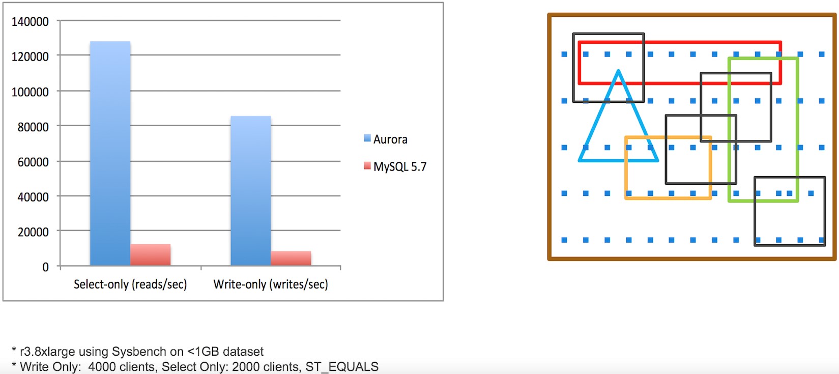
If you have questions, leave a comment here or ping us at aurora-pm@amazon.com.
About the Author
 Sirish Chandrasekaran is a product manager for Amazon Aurora at Amazon Web Services.