AWS Quantum Technologies Blog
Using embedded simulators in Amazon Braket Hybrid Jobs
Today, we launched a new feature in Amazon Braket Hybrid Jobs, which allows you to run hybrid workloads with simulators that are embedded with your algorithm code. For instance, one of the simulators available in this new feature is the PennyLane Lightning GPU simulator, accelerated by NVIDIA’s cuQuantum library. In this blog post, we show you how to get started with a “Hello, world” example, and demonstrate some advanced features, such as how to parallelize quantum machine learning workloads across multiple GPU instances for state-of-the-art performance.
Introduction
Hybrid quantum-classical algorithms, which combine classical and quantum compute resources to iteratively find solutions to computational problems, are a popular approach to near-term quantum computing. In this approach, a parameterized quantum circuit is iteratively adjusted based on intermediate results from a quantum processing unit (QPU) in a classical optimization loop, similar to the training of machine learning models. Researchers in academia and industry are studying the properties of their algorithms in order to answer important questions about the scaling and convergence behavior under different conditions. Since current generation QPUs are limited in their size and coherence, simulators are an important tool for researchers, not only for testing and debugging, but also to study new approaches under ideal conditions, as well as with controlled noise parameters.
With last year’s launch of Hybrid Jobs, we have introduced a framework for the execution of hybrid quantum algorithms on Amazon Braket. As part of your job, you can select any of Braket’s QPUs or on-demand simulator devices, including SV1, DM1, and TN1, to execute the quantum circuits of your hybrid algorithm. With today’s launch, you can now also select embedded simulators for this purpose, where the simulation is part of the algorithm code and executed on the job instance directly. By bringing the simulation closer to your algorithm, you can reduce the latency overhead of communicating with a remote device, which can be a bottleneck for workloads with low qubit numbers (typically up to ~20-25 qubits). Embedded simulators also allow for advanced simulation strategies, such as adjoint differentiation for more efficient gradient computations. Lastly, through the Bring Your Own Container (BYOC) feature, you can experiment with and develop other open source simulation libraries.
Let’s have a look how you can get started with embedded simulators in Braket Hybrid Jobs!
“Hello, world” example – getting started with embedded simulations
Braket Hybrid Jobs helps you to run quantum-classical algorithms more efficiently and with less effort. The first thing we need is an algorithm script in the form of a Python file that defines what you want to run. Let’s start with a “Hello, world” example from PennyLane, that iteratively rotates a single qubit in a pre-defined direction in a variational approach. The algorithm script (hello_world.py) looks like this:
import os
from braket.jobs.metrics import log_metric
from braket.jobs import save_job_result
import pennylane as qml
from pennylane import numpy as np
device_string = os.environ["AMZN_BRAKET_DEVICE_ARN"]
device_prefix = device_string.split(":")[0]
# Boiler plate to set up a device
if device_prefix=="local":
prefix, device_name = device_string.split("/")
device = qml.device(device_name, wires=1)
else:
device = qml.device('braket.aws.qubit',
device_arn=device_string,
wires=1)
# Define the loss function
@qml.qnode(device)
def cost_function(params):
qml.RX(params[0], wires=0)
qml.RY(params[1], wires=0)
return qml.expval(qml.PauliZ(0))
# Initialize and optimize the parameters
params = np.array([0.1, 0.2], requires_grad=True)
opt = qml.GradientDescentOptimizer(stepsize=0.1)
for i in range(5):
params, cost = opt.step_and_cost(cost_function, params)
log_metric(metric_name="Cost", value=cost, iteration_number=i)
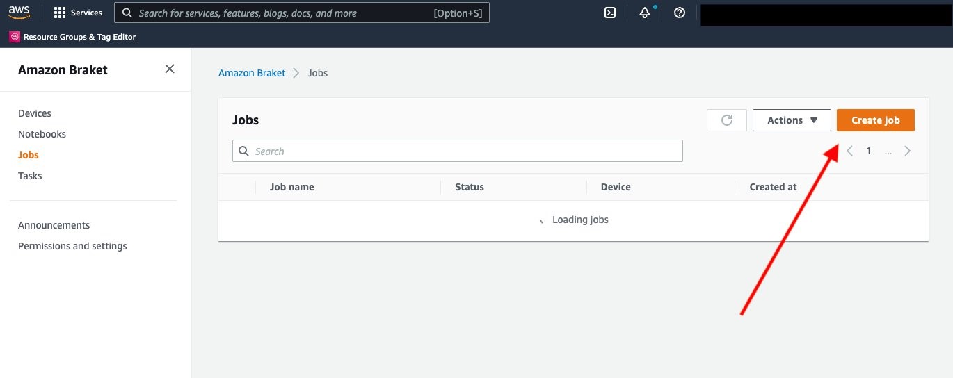
save_job_result({"params": params.tolist()})The boilerplate code after the import commands allows you to programmatically switch between QPUs, on-demand simulators, and PennyLane simulators when creating the job. Now that you have your algorithm script, you can run the job directly from the Braket Hybrid Jobs Console. First navigate to the Jobs tab, and then click on “Create job”:
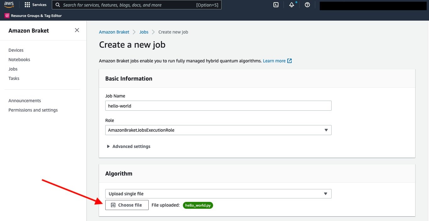
 On the next page, you configure your job. After giving your job a name (‘hello-world’), you can upload your algorithm script, hello_world.py, in the interface here.
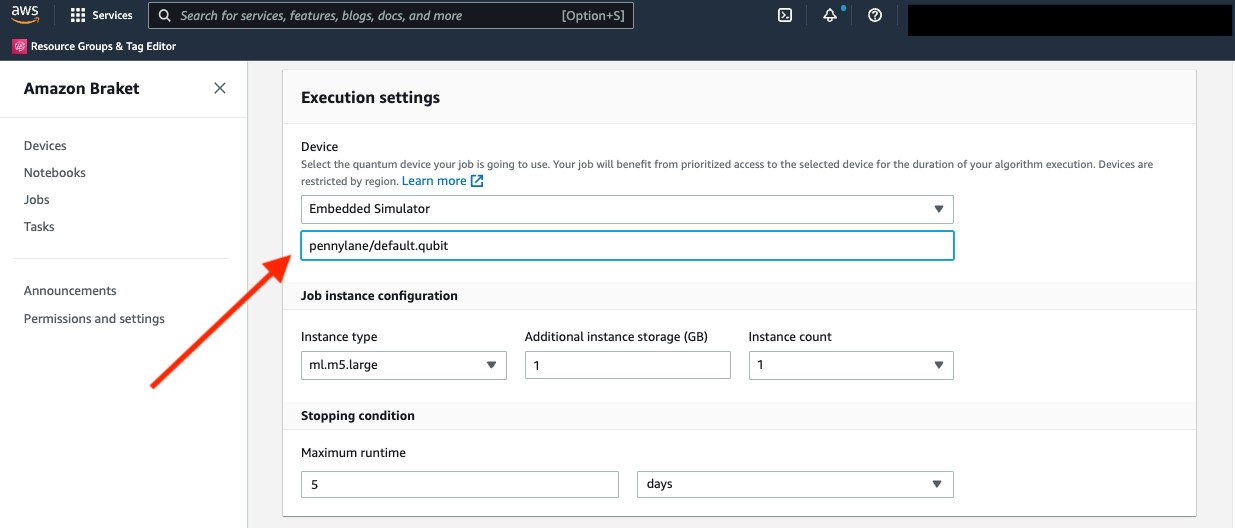
So far, this is the usual experience of Braket Hybrid Jobs. The first difference appears when we select the device. Instead of a QPU or on-demand simulator, we now choose “embedded simulator” in the drop-down menu, and specify the provider and simulator name. For this example we select PennyLane’s default simulator, pennylane/default.qubit.
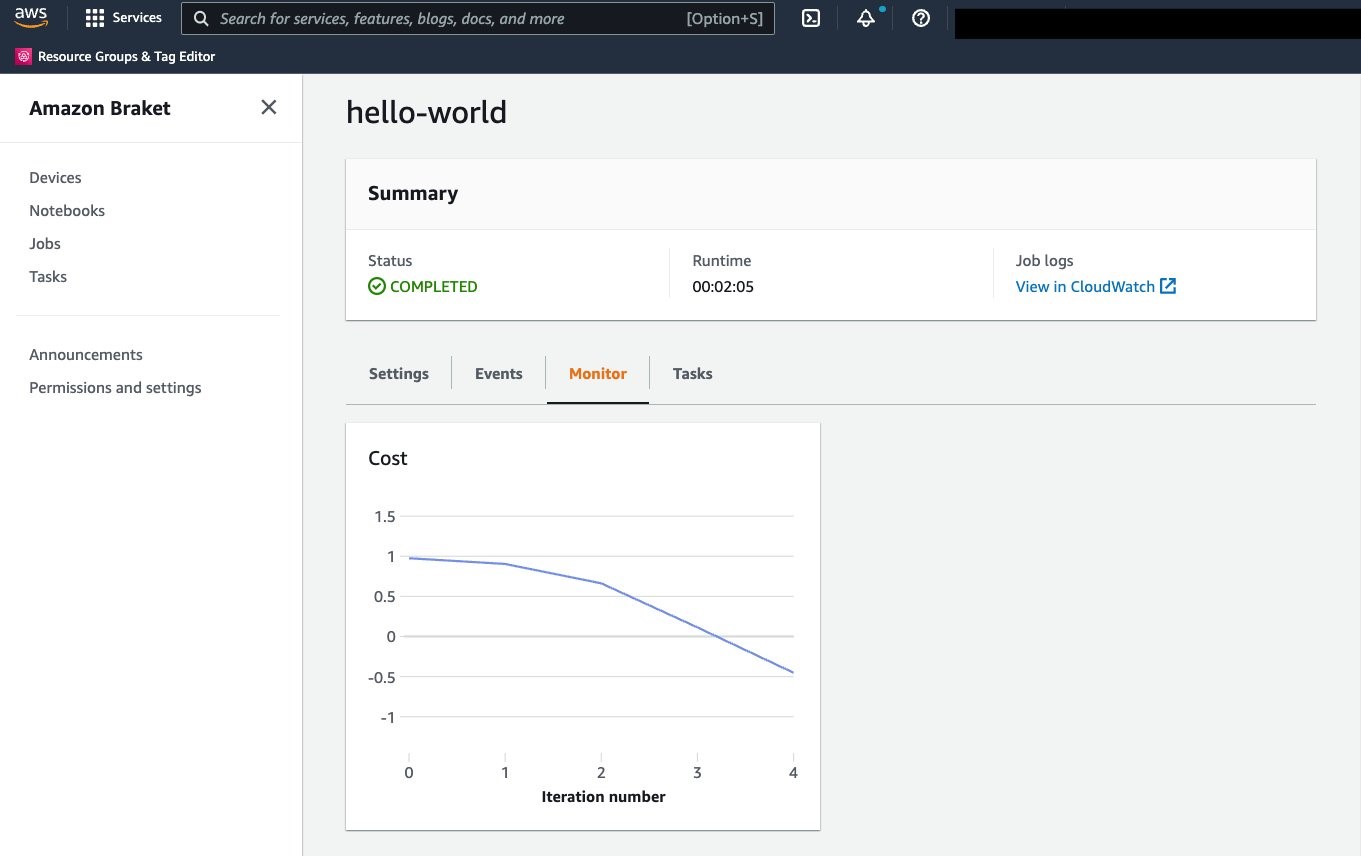
There are more settings you can customize, but for now, we just leave everything as default and click create. Amazon Braket will now spin up the job instance and run your algorithm script. In a few minutes, you can see how your algorithm converges to the solution on the Monitor tab.
This example illustrates how to use embedded simulators, but generally we don’t recommend using Braket Hybrid Jobs for such a small workload, since it takes longer to provision the job instance (a few minutes) than it takes the algorithm to run. It is often easier to run examples like this directly in a Braket notebook or to use local mode. Now let’s take off the training wheels and look at a more advanced example that better illustrates the advantages of embedded simulators.
Quantum machine learning with PennyLane Lightning
In this next example, we will look at a binary classification problem on the Sonar dataset from the UCI repository. The Sonar dataset has 208 data points, each with 60 features that are collected from sonar signals bouncing off materials. Each data point is either labeled as “M” for mines or “R” for rocks. The QML model consists of an input layer, a quantum layer, and an output layer. The input and output layer are classical neural nets implemented in PyTorch. The quantum layer consists of a parameterized quantum circuit which is integrated in the PyTorch code using PennyLane’s qnn module. With a quantum circuit of N qubits, there are 132*N+5 variational parameters in the quantum layer. The cost function is the margin loss function, and the Adam optimizer is used for optimization. The implementation can be found in the algorithm script of this notebook example.
In the “Hello, world” example above, we showed you how to create a job in the console. But you can also create jobs programmatically using the Amazon Braket SDK, e.g., from a Braket notebook or your local IDE. To create a job, you call AwsQuantumJob.create and specify the algorithm script, device, and other configurations through the keyword arguments as shown in the code below.
instance_config = InstanceConfig(instanceType='ml.m5.2xlarge')

hyperparameters={"nwires": "20",
                 "ndata": "208",
                 ...
}

job = AwsQuantumJob.create(
    device="local:pennylane/lightning.qubit",
    source_module="qml_script",
    entry_point="qml_script.train_single",
    input_data={"input-data": "data/sonar.all-data"},
    hyperparameters=hyperparameters,
    instance_config=instance_config,
    image_uri=retrieve_image(Framework.PL_PYTORCH, region)
)
The QML algorithm consists of several python files, so you set source_module to be the local folder containing these files, and set the entry_point to be the file that starts the workload.
Let’s first run the job with lightning.qubit, PennyLane’s CPU-based state vector simulator, on a single m5.2xlarge instance. The m5.2xlarge instance type is comparable to a standard developer laptop. The instance type is specified through the instance_config argument as shown above, and the simulator through the device argument with the format local:<provider>/<simulator_name>. The Sonar dataset, which is the input data, is specified in the input_data argument by its local path. You can also define hyperparameters that are required by your algorithm script. These are parameters that you may want to tune during the experiments, such as the learning rate or the number of qubits in the quantum layer. Because the algorithm uses PyTorch, image_uri is set to be the URI of Braket’s pre-configured PyTorch container image. When you run this code, Amazon Braket will spin up the requested instance, load the dataset onto the instance, and run the algorithm script. Like in the example before, you can monitor the status and progress of the job in the console. The convergence metric, in this case the training error, is displayed in the monitor tab in real time.
One of the advantages of Braket Hybrid Jobs is that with a few lines of code you can run your code on more powerful instances, such as the p3 instance family which is based on NVIDIA® V100 Tensor Core GPUs. All Braket Job containers come pre-installed with PennyLane’s GPU simulator, lightning.gpu, which uses the NVIDIA cuQuantum library for optimized performance on NVIDIA GPU instances. All you need to do in the code above is to change the instance_config argument to use a GPU instance, e.g., to instanceType='ml.p3.2xlarge', and set the device argument to "local:pennylane/lightning.gpu". The p3.2xlarge instance has a single NVIDIA Volta GPU with 16GB of memory.
The m5.2xlarge instance costs $0.00768 per minute, while the p3.2xlarge instance costs $0.06375 per minute. At first, it looks like the GPU instance is the more expensive choice; however, for the 20-qubit example, the time per epoch is 20x shorter for the GPU compared to the CPU instance (~1 minute compared to ~20 minutes). This translates to a cost of $0.06375 and $0.1536, for GPU and CPU respectively, to train each epoch. Thus, by switching to lightning.gpu with a GPU instance, you not only reduce the run time by about 20x but also save 50% of the cost.
But you can do even better. During the training of the quantum model, the loss function is computed for each data point, and then these individual losses are averaged over the whole dataset as the total loss for gradient computations. The losses are computed serially before averaging, which is time consuming and inefficient, especially when there are hundreds of data points. Because the loss from one data point does not depend on other data points, the losses can actually be evaluated in parallel! This is known as data parallelism. With Amazon SageMaker distributed data parallel library, you can leverage data parallelism to accelerate your training with a few lines of code. Let’s have a look how you can distribute your QML problem across multiple GPUs.
In order to use data parallelism, you need to modify the algorithm script to parallelize your data pipeline and QML model using the built-in functions of the SageMaker distributed data parallel library. To learn more about modifying the algorithm script for data parallelism, see our developer guide on the topic. When you create the job, you also need to enable data parallelism by setting the distribution argument to “data_parallel".
Note that to use data parallelism, you need to select the ml.p3.16xlarge instance type, which has 8 GPUs. If you set instanceCount=1, the workload is distributed across the 8 GPUs. If you set instanceCount to be more than 1, the workload is distributed across the all of the GPUs available in all instances. When using multiple instances, each instance incurs charges based on how much time you use it. For example, if you use four instances, the billable time is four times the run time because there are four instances running your workloads at the same time.
instance_config = InstanceConfig(instanceType='ml.p3.16xlarge',
                                 instanceCount=4,
)

hyperparameters={"nwires": "20",
                 "ndata": "208",
                 ...,
}

job = AwsQuantumJob.create(
    device="local:pennylane/lightning.gpu",
    source_module="source_script",
    entry_point="source_script.train_dp",
    input_data={"input-data": "data/sonar.all-data"},
    hyperparameters=hyperparameters,
    instance_config=instance_config,
    image_uri=retrieve_image(Framework.PL_PYTORCH, region)
    distribtion="data_parallel"
)
In the job creation, train_dp.py is the modified algorithm script for using data parallelism. Keep in mind that data parallelism only works correctly when you modify your algorithm script according to the developer guide. If the data parallelism option is enabled without a correctly modified algorithm script, the job may throw errors, or each GPU may repeat the same workload without data parallelism.
We trained the quantum model with qubit counts from 18 to 26 and compared the run time and cost per epoch for different instance configurations: (1) a single ‘laptop-like’ CPU instance (ml.m5.2xlarge), (2) a single GPU instance (ml.p3.2xlarge), (3) a single instance with 8 GPUs (ml.p3.16xlarge), and (4) four instances with 8 GPUs each (ml.p3.16xlarge).
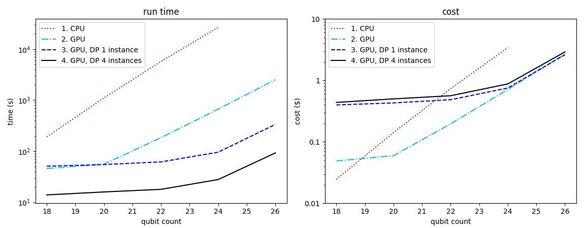
Figure 1: Run time (left) and cost (right) of training the quantum model for an epoch. The CPU instance is m5.2xlarge ($0.00768/min), and the GPU instance is p3.2xlarge ($0.06375/min) for curve 2 and p3.16xlarge ($0.4692/min) for curve 3 and 4. The cost is defined as run time x instance count x cost-per-minute. For curves 3 and 4, the data parallelism (DP) is enabled on one and four instances respectively.
Let’s compare the run time and cost to train the model with 24 qubits. It takes lightning.qubit (CPU-based) about 7.5 hours and about $3.46 to train one epoch (i.e., over 208 data points). For lightning.gpu (GPU-based), without data parallelism, it takes about 10 minutes and $0.64 per epoch. With data parallelism across 4 instances, it only takes lightning.gpu about 30 seconds per epoch, which translates to about $0.94 per epoch. By switching from the CPU simulator in a single instance to parallelized training with the GPU simulator, we improve the run time by about 900x and reduce the cost by about 3.5x.
Conclusion
In this blogpost, we showed you how to simulate hybrid quantum-classical workloads with embedded simulators though the Braket Hybrid Jobs console page, and programmatically through the Amazon Braket SDK. Using a quantum machine learning workload as an example, we showed you how to use PennyLane’s lightning.gpu simulator to accelerate training and save costs. With data parallelism, the training can be sped up further by distributing the workload across multiple GPUs. To learn more and get started with data parallelism, see our developer guide and example notebooks.