AWS Big Data Blog
Close the customer journey loop with Amazon Redshift at Equinox Fitness Clubs
Clickstream analysis tools handle their data well, and some even have impressive BI interfaces. However, analyzing clickstream data in isolation comes with many limitations. For example, a customer is interested in a product or service on your website. They go to your physical store to purchase it. The clickstream analyst asks, “What happened after they viewed the product?” and the commerce analyst asks themselves, “What happened before they bought it?”
It’s no surprise that clickstream data can enhance your other data sources. When used with purchase data, it helps you determine abandoned carts or optimize marketing spending. Similarly, it helps you analyze offline and online behavior, and also behavior before customers even registered an account. However, once the benefits of clickstream data feeds are evident, you must accommodate new requests quickly.
This blog post shows how we, at Equinox Fitness Clubs, moved our data from Amazon Redshift to Amazon S3 to use a late-binding view strategy with our clickstream data. Expect such fun things as Apache Spark, Apache Parquet, data lakes, hive partitioning, and external tables, all of which we will talk about extensively in this post!
When we first started passing our clickstream data from its own tool to our Amazon Redshift data warehouse, speed was the primary concern. Our initial use case was to tie Salesforce data and Adobe Analytics data together to get a better understanding about our lead process. Adobe Analytics could tell us what channel and campaigns people came from, what pages they looked at during the visit, and if they submitted a lead form on our site. Salesforce could tell us if a lead was qualified, if they ever met an advisor, and ultimately if they became a member. Tying these two datasets together helped us better understand and optimize our marketing.
To begin, we knew the steps involved to centralize Salesforce and Adobe Analytics data into Amazon Redshift. However, even when joined together in Redshift, they needed a common identifier to talk to each other. Our first step involved generating and sending the same GUID to both Salesforce and Adobe Analytics when a person submitted a lead form on our website.

Next, we had to pass Salesforce data to Redshift. Luckily, those feeds already existed, so we could add this new GUID attribute in the feed and describe it in Redshift.
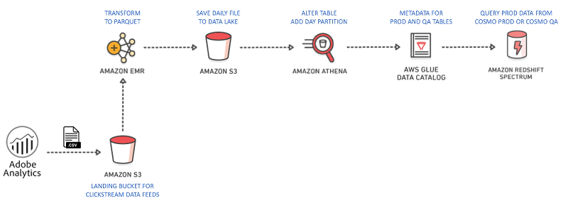
Similarly, we had to generate data feeds from Adobe Analytics to Amazon Redshift. Adobe Analytics provides Amazon S3 as a destination option for our data, so we passed the data to S3 and then created a job to send it to Redshift. The job involved taking the daily Adobe Analytics feed – which comes with a data file containing hundreds of columns and hundreds of thousands of rows, a collection of lookup files like the headers for the data, and a manifest file that describes the files that were sent – and passing it all to Amazon S3 in its raw state. From there, we used Amazon EMR with Apache Spark to process the data feed files into a single CSV file, and then save it to S3 so that we could perform the COPY command to send the data to Amazon Redshift.
The job ran for a few weeks and worked well until we started to use the data more frequently. While the job was effective, backdating data with new columns (schema evolution) started to occur. That’s when we decided we needed greater flexibility because of the nature of the data.
Data lake to the rescue
When we decided to refactor the job, we had two things lined up for us. First, we were already moving towards more of a data lake strategy. Second, Redshift Spectrum had been recently released. It would enable us to query these flat files of clickstream data in our data lake without ever having to run the COPY command and store it in Redshift. Also, we could more efficiently join the clickstream data to other data sources stored inside of Redshift.

We wanted to take advantage of self-describing data which combines the schema of the data with the data itself. Converting the data to self-describing data would help us manage the wide clickstream datasets and prevent the schema-evolution related challenges. We could pull every column we desired into the data lake file and then use only the important columns in our queries to speed up processing. To accomplish this flexibility, we used the Apache Parquet file format, which is both self-describing and blazing fast due to its columnar storage technology. We used Apache Spark on Amazon EMR to convert from CSV to Parquet, and partition the data for scanning performance, as shown in the following code.
Using the AWS Glue Data Catalog allowed us to make our clickstream data available to be queried within Amazon Redshift and other query tools like Amazon Athena and Apache Spark. This is accomplished by mapping the Parquet file to a relational schema. AWS Glue, enables querying additional data in mere seconds. This is because schema changes can occur in real time. This means you can delete and add columns, reorder column indices, and change column types all at once. You can then query the data immediately after saving the schema. Additionally, Parquet format prevents failures when the shape of the data changes, or when certain columns are deprecated and removed from the data set.
We used the following query to create our first AWS Glue table for our Adobe Analytics website data. We ran this query in Amazon Redshift in SQL Workbench.
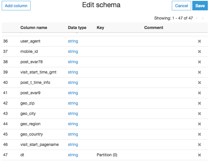
After running this query, we added additional columns to the schema upon request throughthe AWS Glue interface. We also used partitioning to make our queries faster and cheaper.

At this point, we had a new schema folder in our database. It contained the external table that could be queried, but we wanted to take it a step further. We needed to add some transformations to the data such as:
- Renaming IDs to strings
- Concatenating values
- Manipulating strings, excluding bot traffic that we send from AWS to test the website
- Changing the column names to be more user friendly.
To do this, we created a view of the external table, as follows:
Now we can perform queries from Amazon Redshift, blending our structured Salesforce data with our semi-structured, dynamic Adobe Analytics data. With these changes, our data became extremely flexible, friendly on storage size, and very performant when queried. Since then, we have started using Redshift Spectrum for many use cases from data quality checks, machine data, historical data archiving, and empowering our data analysts and scientists to more easily blend and onboard data.
Conclusion
We were able to setup an efficient and flexible analytics platform for clickstream data by combining the Amazon S3 data lake with Amazon Redshift. This has eliminated the need to always load clickstream data into the data warehouse, and also made the platform adaptable to schema changes in the incoming data. You can read the Redshift documentation to get started with Redshift Spectrum, and also watch our presentation at the AWS Chicago Summit 2018 below.
Additional Reading
If you found this post helpful, be sure to check out From Data Lake to Data Warehouse: Enhancing Customer 360 with Amazon Redshift Spectrum, and Narrativ is helping producers monetize their digital content with Amazon Redshift.
About the Author
 Ryan Kelly is a data architect at Equinox, where he helps outline and implement frameworks for data initiatives. He also leads clickstream tracking which helps aid teams with insights on their digital initiatives. Ryan loves making it easier for people to reach and ingest their data for the purposes of business intelligence, analytics, and product/service enrichment. He also loves exploring and vetting new technologies to see how they can enhance what they do at Equinox.