AWS Big Data Blog
Maximize data ingestion and reporting performance on Amazon Redshift
This is a guest post from ZS. In their own words, “ZS is a professional services firm that works closely with companies to help develop and deliver products and solutions that drive customer value and company results. ZS engagements involve a blend of technology, consulting, analytics, and operations, and are targeted toward improving the commercial experience for clients.”
ZS was involved in setting up and operating a MicroStrategy-based BI application that sources 700 GB of data from Amazon Redshift as a data warehouse in an Amazon-hosted backend architecture. ZS sourced healthcare data from various pharma data vendors from different systems such as Amazon S3 buckets and FTP systems into the data lake. They processed this data using transient Amazon EMR clusters and stored it on Amazon S3 for reporting consumption. The reporting-specific data is moved to Amazon Redshift using COPY commands, and MicroStrategy uses it to refresh front-end dashboards.
ZS has strict, client-set SLAs to meet with the available Amazon Redshift infrastructure. We carried out experiments to identify an approach to handle large data volumes using the available small Amazon Redshift cluster.
This post provides an approach for loading a large volume of data from S3 to Amazon Redshift and applies efficient distribution techniques for enhanced performance of reporting queries on a relatively small Amazon Redshift cluster.
Data processing methodology
ZS infrastructure is hosted on AWS, where they store and process pharma industry data from various vendors using AWS services before reporting the data on a MicroStrategy BI reporting tool. The following diagram shows the overall data flow from flat files to reports shown on MicroStrategy for end-users.
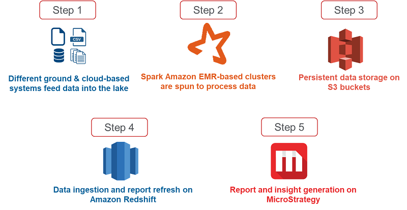
Step 1: Pharma data is sourced from various vendors and different systems like FTP location, individual systems and Amazon S3 buckets etc.
Step 2: Cost-effective transient clusters are spun as needed to provide compute power to execute pyspark codes.
Step 3: Post the processing, data is stored in Amazon S3 buckets for consumption of downstream applications.
Step 4: 700 GB of data is then ingested into Amazon Redshift for MSTR consumption.
Step 5: This data is read from Amazon Redshift and the insights are displayed to the end-users in the form of reports on MicroStrategy.
Dataset under consideration
In this specific scenario, ZS was working with data from the pharma domain. The following table demonstrates the data’s typical structure—it has several doctor, patient, treatment-pertinent IDs, and healthcare metrics.
| Table 1 | ||
| Column Name | EMR datatype | Amazon Redshift datatype |
| Time ID | integer | int |
| Geography ID | integer | int |
| Product ID | integer | int |
| Market ID | integer | int |
| Doctor ID | integer | int |
| Doctor Attribute 1 ID | integer | int |
| Doctor Attribute 2 ID | integer | int |
| Doctor Attribute 3 ID | integer | int |
| Doctor Attribute 4 ID | integer | int |
| Doctor Rank | integer | int |
| Metric 1 | double | decimal(18,6) |
| Metric 2 | double | decimal(18,6) |
| Metric 3 | double | decimal(18,6) |
| Metric 4 | double | decimal(18,6) |
| Metric 5 | double | decimal(18,6) |
| Metric 6 | double | decimal(18,6) |
| Metric 7 | double | decimal(18,6) |
| Metric 8 | double | decimal(18,6) |
| Metric 9 | double | decimal(18,6) |
| Metric 10 | double | decimal(18,6) |
| Metric 11 | double | decimal(18,6) |
| Metric 12 | double | decimal(18,6) |
| Metric 13 | double | decimal(18,6) |
| Metric 14 | double | decimal(18,6) |
| Metric 15 | double | decimal(18,6) |
| Metric 16 | double | decimal(18,6) |
| Metric 17 | double | decimal(18,6) |
| Metric 18 | double | decimal(18,6) |
| Metric 19 | double | decimal(18,6) |
| Metric 20 | double | decimal(18,6) |
| Metric 21 | double | decimal(18,6) |
| Metric 22 | double | decimal(18,6) |
| Metric 23 | double | decimal(18,6) |
| Data Snapshot Date | timestamp | timestamp |
| Data Refresh Date | timestamp | timestamp |
| Data Refresh ID | string | varchar |
Each table has approximately 35–40 columns and holds approximately 200–250M rows of data. ZS used 40 such tables; they sourced the data in these tables from various healthcare data vendors and processed them as per reporting needs.
The total dataset is approximately 2 TB in size in CSV format and approximately 700 GB in Parquet format.
Challenges and constraints
The five-step process for data refresh and insight generation outlined previously takes place over the weekends within a stipulated time frame. Under default, unoptimized state data load from S3 to Amazon Redshift and MicroStrategy refresh (Step 4 in the previous diagram) took almost 13–14 hours on a 2node ds2.8xlarge cluster and was affecting the overall weekend run SLA (1.5 hours).
The following diagram outlines the three constraints that ZS had to solve for to meet client needs:

Weekly time-based SLA – Load within 1 hour and fetch data on MSTR within 1.5 hours
The client IT and Business teams set a strict SLA to load 700 GB of Parquet data (equivalent to 2 TB CSV) onto Amazon Redshift and refresh the reports on the MicroStrategy BI tool. In this scenario, the client team had moved from another vendor to AWS, and the overall client expectation was to reduce costs without a significant performance dip.
Fixed cluster size – Pre-decided 2 node ds2.8xlarge cluster
The client IT teams determined the cluster size and configuration, and took into consideration the cost, data volumes, and load patterns. These were fixed and not adjustable: a 2 node ds2.8xlarge cluster. ZS carried out PoCs to optimize the environment subject to these constraints.
High data volume – Truncate load 700GB data in Parquet format
The data that ZS used was pertinent to the Pharma domain. The dataset under consideration in this scenario was 700 GB in Parquet format. In this specific use case, with every refresh, even historic data was updated, and therefore a lot of data could not be appended. Therefore, we followed a truncate and load process.
Iterative optimization
With constraints over time, data volume, and cluster size, ZS performed various experiments to optimize Amazon Redshift data load and read time—two key aspects to gauge performance. ZS created an iterative framework that helps do the following:
- Decide the file format
- Define optimal data distribution through distribution and sort keys
- Identify the techniques to parallelize the data-loading process
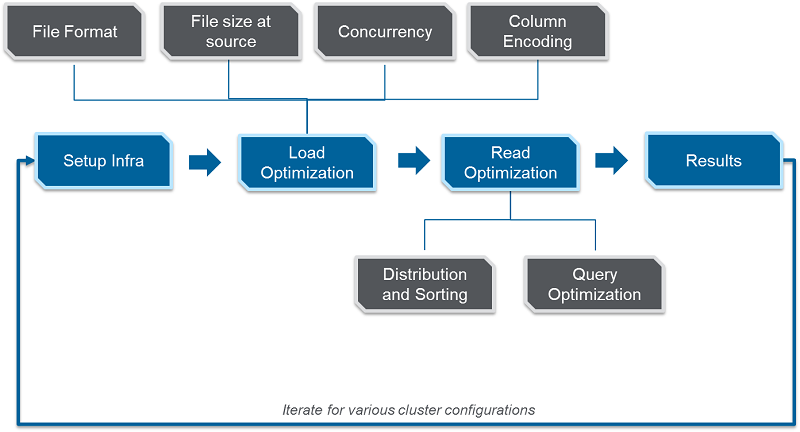
The below diagram shows the key steps that can be followed to get the best data load and read performance on any Amazon RedShift cluster.
Data load optimization
We identified and optimized four key factors impacting data load performance: file formats, file size at source, concurrency, and column encoding.
File formats
Many projects usually load data in CSV format from S3 to Amazon Redshift. ZS had data available in Parquet format with snappy compression as an output of Spark processes. (Spark processes work best with this combination.)
To identify an efficient format for Amazon Redshift, we compared Parquet with commonly used CSV and GZIP formats. We loaded a table from S3, with 200M rows of data generated through the Spark process, which equates to 41 GB in CSV, 11 GB in Parquet, and 10 GB in GZIP, and compared load time and CPU utilization. The below diagram shows load time vs CPU utilization for same data stored in different file formats.
For the dataset and constraints we were working with, loading the Parquet format file required low CPU utilization and lesser I/O compared to CSV and GZIP, and occupied a smaller memory footprint on S3 compared to the memory-intensive CSV format. Lower CPU utilization allowed more parallel loads in this scenario, thereby reducing the overall runtime required to load Parquet files.

File size at source
The next aspect was to choose the block size in which the Parquet files were broken down and stored on S3. A block size of 128 MB is commonly used for Spark jobs and considered to be optimal for data processing. However, Amazon Redshift works best with larger files.
We loaded 10 GB of Parquet data broken down into smaller equisized files of 250 MB, 750 MB, 1 GB, 1.5 GB, and 3 GB block sizes and noted the performance in each case. The following graph shows the different load times.
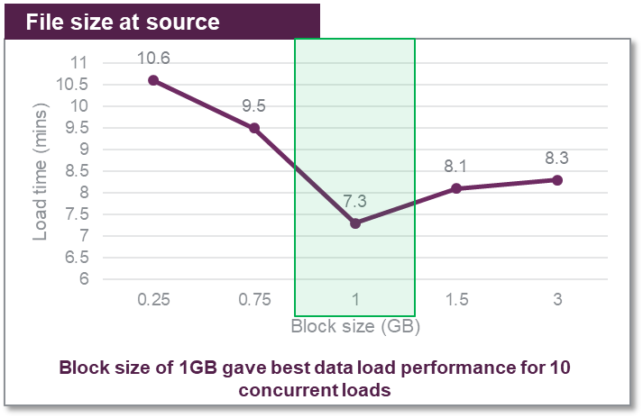
There was a gradual improvement in the data load time until the block size reached 1 GB (with best load timing). Beyond 1GB mark there was a dip in performance observed with larger files and Amazon Redshift took more time to process larger files.
These numbers are specific to the kind of data we were working with. The recommendations can vary as the form and shape of data changes.
As a best practice, identify the block size and have the number of files as a multiple of the number of slices of the Amazon Redshift cluster. This makes sure that each slice does an equal amount of work and there are no idle slices, thereby increasing efficiency and improving performance. For more information, see Top 8 Best Practices for High-Performance ETL Processing Using Amazon Redshift.
Concurrency
The COPY command is relatively low on memory. The more parallel the loads, the better the performance. ZS loaded a table approximately 7.3 GB multiple times with separate concurrency settings. We measured the throughput in terms of the average time taken per GB to move files to Amazon Redshift with 1 to 20 concurrent loads. The following table summarizes the results.
| Test | Number of tables loaded in parallel (concurrency) | Total data loaded (GB) |
| Test 1 | 1 | 7.3 |
| Test 2 | 5 | 36.5 |
| Test 3 | 10 | 73 |
| Test 4 | 15 | 109.5 |
| Test 5 | 20 | 146 |
The below diagram shows the time taken to load 1GB of data and the CPU utilization for various concurrency settings.
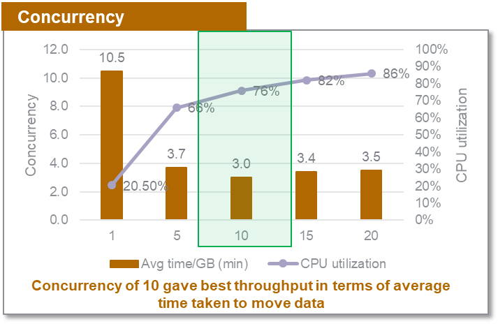
For the dataset and constraints we were working with, a concurrency of 10 gave the best throughput for our specific dataset, with a 25% CPU availability buffer of about 25%. Depending on the nature of the data and volume fluctuations every release, you can opt for a different buffer.
Column encoding
To identify the column encoding and compression on Amazon Redshift that gives the best performance and occupies lower storage footprint, ZS compared ZSTD (which the ANALYZE COMPRESSSION command recommended), LZO, and none encoding formats on Amazon Redshift tables for load performance. The below diagram shows the time taken to load same data volume into the tables with none, ZSTD and LZO encoding applied to the columns.
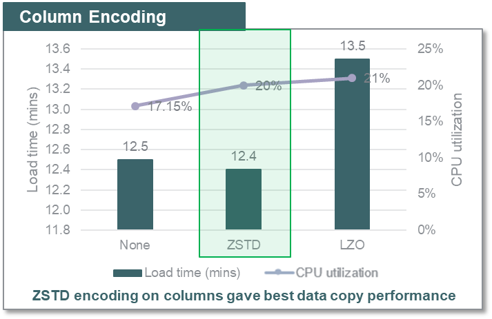
For the dataset and constraints we were working with, ZSTD encoding on columns offered a high compression ratio (~3, than when there was no compression used) and gave the best data copy performance and low storage footprint on Amazon Redshift for our use case. You can have varied results depending on the datatype and cardinality of the data.
Note: This solution was implemented prior to the feature release for AZ64 encoding and hence does not consider its impact. One could use the approach described in this blog post considering AZ64 compression encoding among all the compression encodings Amazon Redshift supports.
Data read optimization
ZS also improved the data read performance by MicroStrategy from Amazon Redshift by using distribution and sorting keys and SQL optimization (minimizing filters on MicroStrategy auto-generated SQL queries).
SQL queries
MicroStrategy is a business intelligence tool and reads data from a database by intelligently building its own SQL. We compared the performance of MSTR SQLs (typical DW queries such as SELECT, GROUP BY, or temporary tables) with and without filters and observed that the query with and without filters for our dataset ran in almost the same time and used the same resources. But the unfiltered query gave four times more data. The following table summarizes the results.
|
Filters? |
Rows fetched | Query runtime | CPU utilization |
|
Y |
500K |
5.1 (mins) |
15% |
| N | 2M | 5.1 (mins) |
15% |
Tweaking the SQLs to have minimum or no filters can help fetch significantly more rows with only a small increase in processing time, compared to what it takes to read data with more filters. If you need to use the entire dataset, it is better to fetch complete data using one query than using several SQLs with separate filters and running them in parallel.
Distribution and sort keys
The following table is an analysis of a table load and read performance with and without distribution and sort keys for our use case.
| Dist. Style | Dist Key | Sort Keys | Load time (mins) | Query run time (mins) | Query CPU utilization |
| None | – | – | 16.7 | 59.5 | 59% |
| Key | Most suitable distribution key depending on the query that gives even distribution | 6 columns that appear in where clause, in the order of group by clause in SQL | 17.5 | 36.1 | 32% |
The table without a distribution key loaded a little faster. However, differences in data read time and CPU utilization between the two queries is significant. This means that more and more parallel loads could run efficiently when the keys were set appropriately, because the overall CPU utilization reduced significantly. The key takeaway is to use a distribution style—auto, even, or manual—to optimize data read from Amazon Redshift and allow more parallel processing. ZS used a manual distribution style and chose distribution and sort keys based on an extensive understanding of data and refresh cadence.
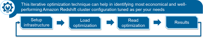
Next steps to get the best output from your Amazon Redshift instance
As an outcome of the multiple POC results, we identified the most suitable file formats, compression techniques, re-partitioned Parquet file block sizes, and distribution and interleaved sorting logic that offer the best performance for our dataset for reporting on MicroStrategy with Amazon Redshift as the database. This helped us identify the best data load and read combinations to load 700 GB of Parquet data (equivalent to 2 TB of CSV data) within the client-set 2.5 hour SLA using the available fixed 2 node ds2.8xlarge cluster.
The following diagram shows the iterative process you can follow to identify the best data load and read techniques suited for an Amazon Redshift cluster configuration.
The following are a few key takeaways:
- Parquet and Amazon Redshift worked well together. The data in Parquet format had low CPU utilization and I/O requirements, which allowed more parallel loads.
- ZSTD encoding worked best for this specific dataset due to encoding on numbers as well.
- Sort keys and distribution keys on tables can bring down read time by approximately 80% compared to tables with no distribution and sorting logic applied.
- Filtering data on Amazon Redshift does not work the same as typical databases. You can improve data filtering performance with the appropriate sort keys.
- File size at the source and concurrency are interrelated and you should choose them accordingly. Larger blocks (maximum 1 GB, for this specific dataset) are loaded faster onto Amazon Redshift.
About the Authors
 Vasu Kiran Gorti is a result-oriented professional with technology and functional/domain experience predominantly in sales and marketing consulting. Essaying a role of Associate Consultant at ZS Associates, he has experience in working with life sciences and healthcare clients in alignment to their business objectives and expectations. He specializes in MicroStrategy, Business Intelligence, Analytics, and reporting. Proactive and innovative, Vasu enjoys taking up stimulating initiatives that bridge the gap between technology and business. He’s a permanent beta—always learning, improvising and evolving.
 Ajit Pathak is a Technology Consultant at ZS Associates and leads BI and data management projects for Pharmaceutical companies. His areas of interest and expertise include MSTR, Redshift, and AWS suite. He loves designing complex applications and recommending best architectural practices that lead to efficient and concise dashboards. A qualified technology consultant, Ajit has focused on driving informed business decisions through clear data communication. When he is not focusing on areas of data visualizations and applications, Ajit loves to read, play badminton, and participate in debates ranging from politics to sports.