Improve query performance with EXPLAIN plans in Amazon Aurora DSQL

You’ve migrated to Amazon Aurora DSQL and you’re ready to get the most out of your queries. Whether you’re looking to reduce latency or optimize your Distributed Processing Unit (DPU) costs, understanding how Aurora DSQL runs queries can help you improve performance. The EXPLAIN command follows familiar PostgreSQL conventions, with output designed for readability and a clear mental model. However, the distributed architecture of Aurora DSQL introduces new optimization opportunities that go beyond traditional PostgreSQL tuning techniques.

Amazon Aurora DSQL is a serverless PostgreSQL-compatible database. Aurora DSQL is designed to scale from quick prototypes to the largest active-active single-Region or multi-Region workloads. Its architecture differs from a single-node PostgreSQL instance in ways that create new optimization opportunities: compute and storage are physically separated for independent scaling, primary keys serve as fully covering indexes by default for faster lookups, and query execution spans a disaggregated system where optimizing data movement between layers can yield meaningful performance gains. Because of these differences, EXPLAIN plan output in Aurora DSQL looks familiar while offering richer optimization signals. The plan nodes have new names, filter placement carries real cost impact, and applying a fresh perspective to query tuning can help you achieve better results.

In this post, we show you how to use EXPLAIN plans to diagnose and improve query performance in Amazon Aurora DSQL. We introduce a three-layer filter model as a practical framework for understanding where your predicates are evaluated, and walk through the architecture differences that make Aurora DSQL plans unique, the anatomy of an EXPLAIN output, access method selection, and a step-by-step query improvement workflow.

How Aurora DSQL differs from PostgreSQL (architecture primer)

Before diving into EXPLAIN plans in Amazon Aurora DSQL, it helps to understand why they look different from standard PostgreSQL plans. You don’t need a deep infrastructure background. A clear mental model of two key differences is all it takes to make every EXPLAIN plan immediately more readable.

Key difference 1: No heap storage—the primary key is the table

In standard PostgreSQL, tables are stored as heaps, which are unordered collections of rows in physical pages. Indexes are separate structures that point back to the heap. An Index Scan therefore involves two steps: traverse the index to find matching entries, then follow heap pointers to fetch the full row. Index Only Scans exist as a separate, more efficient operation because they avoid the heap fetch entirely when all needed columns are in the index.

In Amazon Aurora DSQL, there is no heap storage. Every table is stored as a B-tree index organized by the primary key. The primary key isn’t a pointer to data. It’s the data. If you don’t define a primary key explicitly, Amazon Aurora DSQL assigns a hidden, system-generated ID to maintain this structure. Several implications follow from this design:

• Queries against tables without a user-defined primary key produce Full Scans rather than Sequential Scans, a different operation with different cost characteristics.
• Secondary indexes in Amazon Aurora DSQL always carry the primary key columns implicitly, which affects how the optimizer chooses between index paths.
• In standard PostgreSQL, an Index Scan is a single plan node, and the heap fetch is implicit and invisible in the EXPLAIN output. In Amazon Aurora DSQL, the Storage Lookup is an explicit, separate node with its own cost estimates, row counts, and loop counts.

Design consideration: Because the primary key is a full covering index, a well-chosen key can deliver real performance benefits from day one. This makes primary key selection a high-impact design opportunity in Aurora DSQL compared to PostgreSQL. Choose natural keys that match your dominant access pattern over synthetic surrogate keys, when uniqueness and stability permit.

Key difference 2: Compute and storage are physically separated

In Amazon Aurora DSQL, the query processor (compute) and the storage layer are distinct, networked components. Every byte of data that travels from storage to the query processor has a real cost in latency and Distributed Processing Unit (DPU) consumption, which measures the compute and I/O resources consumed by each query. This separation is what makes filter pushdown a performance-critical decision in ways that it’s not in PostgreSQL.

In standard PostgreSQL, a filter applied in memory after a heap fetch has minimal performance impact because data is local. In Amazon Aurora DSQL, when the query processor applies a filter, all unfiltered data has already crossed the network from storage. Pushing filters down to the storage layer or, better, to the index condition level is the primary lever for Amazon Aurora DSQL query optimization.

PostgreSQL and Aurora DSQL: key architecture differences

Prerequisites

To follow along with the examples in this post, you need:

• An active AWS account with permissions to create Amazon Aurora DSQL clusters (dsql:CreateCluster, dsql:GetCluster, dsql:GenerateDbConnectAdminAuthToken)
• AWS Command Line Interface (AWS CLI) v2 with Aurora DSQL support (aws dsql commands available)
• A PostgreSQL-compatible client such as psql 16 or later
• Basic familiarity with SQL queries and EXPLAIN plan output

To create an Aurora DSQL cluster and connect, refer to Getting started with Aurora DSQL. Alternatively, you can use the Aurora DSQL Playground to run the examples in this post without provisioning your own cluster.

The examples in this post use three tables: transaction, account, and customer. Create the full schema by running the following statements against your Aurora DSQL cluster:

CREATE TABLE customer (
    customer_id  uuid PRIMARY KEY,
    name         varchar,
    region       varchar
);

CREATE TABLE account (
    customer_id  uuid,
    balance      numeric,
    status       varchar,
    created_at   timestamp
);

CREATE TABLE transaction (
    account_id        uuid,
    customer_id       uuid,
    transaction_date  timestamp,
    description       text
);

-- Index on account: covers customer_id, balance, status but NOT created_at
CREATE INDEX ASYNC idx1 ON account (customer_id) INCLUDE (balance, status);

-- Indexes for join optimization examples (Pattern 4)
CREATE INDEX ASYNC idx_account_customerid ON account (customer_id);
CREATE INDEX ASYNC idx_transaction_customerid ON transaction (customer_id);

The transaction table intentionally has no explicitly defined primary key. When you omit a primary key, Amazon Aurora DSQL assigns a hidden, system-generated ID to each row to maintain its internal B-tree structure. This forces Full Scan behavior so you can observe the impact of adding an index later. The idx1 index on account intentionally excludes created_at so you can observe Storage Lookup behavior when that column is queried. The customer table and its related indexes are used in the join optimization examples later in this post.

Next, seed sample data. Amazon Aurora DSQL has a 3,000-row per-transaction mutation limit, so insert in batches:

-- Seed customer table
INSERT INTO customer (customer_id, name, region)
SELECT
    gen_random_uuid(),
    'Customer ' || s,
    CASE (s % 3)
        WHEN 0 THEN 'us-east-1'
        WHEN 1 THEN 'eu-west-1'
        WHEN 2 THEN 'ap-southeast-1'
    END
FROM generate_series(1, 2500) AS s;

-- Seed transaction table (run this insert 10 times to reach 30,000 rows)
INSERT INTO transaction (account_id, customer_id, transaction_date, description)
SELECT
    gen_random_uuid(),
    (SELECT customer_id FROM customer ORDER BY random() LIMIT 1),
    NOW() - ((s % 365) || ' days')::interval - ((s % 24) || ' hours')::interval,
    CASE (s % 10)
        WHEN 0 THEN 'Direct deposit'    WHEN 1 THEN 'Wire transfer'
        WHEN 2 THEN 'ATM withdrawal'    WHEN 3 THEN 'Online purchase'
        WHEN 4 THEN 'Subscription payment' WHEN 5 THEN 'Refund'
        WHEN 6 THEN 'Interest credit'   WHEN 7 THEN 'Fee charge'
        WHEN 8 THEN 'Peer-to-peer transfer' WHEN 9 THEN 'Check deposit'
    END
FROM generate_series(1, 3000) AS s;

-- Seed account table
INSERT INTO account (customer_id, balance, status, created_at)
SELECT
    (SELECT customer_id FROM customer ORDER BY random() LIMIT 1),
    ROUND((random() * 99999.99)::numeric, 2),
    CASE (s % 4)
        WHEN 0 THEN 'active'   WHEN 1 THEN 'inactive'
        WHEN 2 THEN 'pending'  WHEN 3 THEN 'closed'
    END,
    NOW() - ((s % 730) || ' days')::interval - ((s % 24) || ' hours')::interval
FROM generate_series(1, 2500) AS s;

Run the transaction insert 10 times to reach 30,000 rows. Because account_id uses gen_random_uuid(), each execution produces unique rows, so you don’t need to adjust the generate_series range between runs. Run the account insert four times to reach 10,000 rows.

Amazon Aurora DSQL automatically refreshes table statistics as data changes through a probabilistic Auto Analyze mechanism. For this walkthrough, we run ANALYZE manually to produce deterministic plan output for demonstration purposes. In production, Auto Analyze handles this reliably. In our testing, the planner consistently chose the correct plan without manual intervention. To learn more about when and how Auto Analyze triggers, see Auto Analyze in Aurora DSQL.

ANALYZE customer;
ANALYZE transaction;
ANALYZE account;

Test environment: The EXPLAIN plan outputs and DPU measurements in this post were captured on a single-Region Aurora DSQL cluster in us-east-1, with 30,000 rows in the transaction table and 10,000 rows in the account table. Data was inserted in batches of 3,000 rows (Aurora DSQL’s per-transaction row mutation limit). Your actual DPU values and execution times will vary based on data volume, row size, cluster configuration, and query selectivity.

Understanding Amazon Aurora DSQL EXPLAIN plans

Before diagnosing performance problems, let’s look at what each element of an Amazon Aurora DSQL EXPLAIN plan tells you. Each element in the output conveys a specific part of the execution story.

Key elements at a glance

Aurora DSQL scan types: when each appears and what it means

Amazon Aurora DSQL has different scan types. Understanding when each is used, and which one you should be targeting, is the foundation of query optimization in Amazon Aurora DSQL.

1. Full Scan

A Full Scan reads the entire table. The optimizer chooses it when no index can satisfy the query’s filter predicates, either because the table has no usable index, or because the optimizer determines a full scan is cheaper than an index path.

Example: The transaction table has no user-defined primary key and no secondary indexes on transaction_date, so a query filtering on that column produces a Full Scan:

EXPLAIN
SELECT account_id, transaction_date, description
FROM transaction
WHERE transaction_date > '2024-06-01';

Full Scan (btree-table) on transaction  (cost=3850.04..4575.03 rows=29997 width=42)
  -> Storage Scan on transaction  (rows=29997 width=42)
      Projections: account_id, transaction_date, description
      Filters: (transaction_date > '2024-06-01'::timestamp without time zone)
      -> B-Tree Scan on transaction  (rows=30000 width=42)

The transaction_date filter appears as a Storage Filter (Level 2) inside the Storage Scan node. Without an index on transaction_date, the filter can’t be an Index Condition (Level 1), but Amazon Aurora DSQL still pushes it to the storage layer so filtering happens before data is transferred to the query processor. The B-Tree Scan reads all 30,000 rows, and the storage filter reduces the result set before transfer.

2. Index Only Scan

An Index Only Scan is the scan type that you want to see for most queries. It means all data needed by the query, both for filtering and for projection, can be satisfied entirely from the index, without touching the base table. This is the most efficient path and typically involves the fewest storage round trips.

An Index Only Scan is chosen when:

1. All filter predicates are on indexed key columns (so they can be Index Conditions).
2. All projected columns (the SELECT list) are also in the index, either as key columns or INCLUDE columns.

Example: The account table has idx1 on (customer_id) INCLUDE (balance, status). When you query only covered columns, Amazon Aurora DSQL uses an Index Only Scan:

EXPLAIN
SELECT balance
FROM account
WHERE customer_id = '4b18a761-5870-4d7c-95ce-0a48eca3fceb';

Index Only Scan using idx1 on account  (cost=100.16..104.17 rows=1 width=11)
  Index Cond: (customer_id = '4b18a761-...'::uuid)       ← Level 1: Index Condition
  -> Storage Scan on idx1  (cost=100.16..104.17 rows=1 width=11 loops=1)
      Projections: balance
      -> B-Tree Scan on idx1  (cost=100.16..104.17 rows=1 width=11 loops=1)
          Index Cond: (customer_id = '4b18a761-...'::uuid)

The customer_id filter is an Index Condition (Level 1). Amazon Aurora DSQL reads only matching index entries and returns balance directly from the index.

3. Index Scan

An Index Scan in Amazon Aurora DSQL appears when the index can satisfy the query’s filter predicates but not all of its projected columns. The EXPLAIN output makes this visible as two storage operations: a Storage Scan on the index to find matching entries, followed by a Storage Lookup on the base table to fetch the missing columns. In standard PostgreSQL, this base table fetch is implicit within the Index Scan node. In Amazon Aurora DSQL, it’s an explicit node with its own cost and row count, making the overhead directly measurable.

Example: When you select created_at, a column not in idx1, Amazon Aurora DSQL must make an extra round trip to the base table:

EXPLAIN
SELECT balance, status, created_at
FROM account
WHERE customer_id = '4b18a761-5870-4d7c-95ce-0a48eca3fceb';

Index Scan using idx1 on account  (cost=100.28..208.29 rows=1 width=29)
  Index Cond: (customer_id = '4b18a761-...'::uuid)       ← Level 1: Index Condition
  -> Storage Scan on idx1  (cost=100.28..208.29 rows=1 width=29 loops=1)
      -> B-Tree Scan on idx1  (cost=100.28..208.29 rows=1 width=29 loops=1)
          Index Cond: (customer_id = '4b18a761-...'::uuid)
  -> Storage Lookup on account  (cost=100.28..208.29 rows=1 width=29 loops=1)
      Projections: balance, status, created_at            ← Extra round trip for created_at
      -> B-Tree Lookup on account  (cost=100.28..208.29 rows=1 width=29 loops=1)

The Storage Lookup sub-node is the telltale sign: Amazon Aurora DSQL went back to the base table to fetch created_at. The Projections line confirms which columns required the extra round trip.

Scan type quick reference

Note: Adding INCLUDE columns speeds up queries by avoiding the base-table lookup, but there’s a trade-off: each included column is copied into every entry in the index, making the index larger and increasing storage costs. Only include columns that your most important queries actually need.

The three-layer filter model: your optimization compass

The most important mental model for Amazon Aurora DSQL query optimization is the three-layer filter model. Every predicate in your query is evaluated at one of three layers in the execution stack, and the layer where your filter lands directly determines how much data moves through the system.

The goal is to move predicates from Level 3 to Level 2 to Level 1. Each step down the stack reduces the amount of data that crosses the network between storage and compute, directly reducing query latency and DPU consumption.

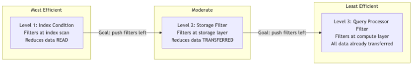
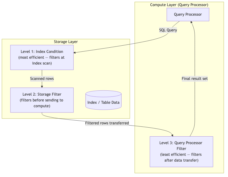
Figure 1: Amazon Aurora DSQL query execution flow showing the three filter levels.

A practical query optimization workflow

Now that you understand the vocabulary and the filter model, here is the end-to-end workflow for diagnosing and fixing a slow query in Amazon Aurora DSQL.

Step 1: Run EXPLAIN (not EXPLAIN ANALYZE) first

For initial diagnosis, start with plain EXPLAIN. This avoids running the query (critically important for expensive queries) and gives you the optimizer’s intended plan. At this stage, look for three things:

• Are your most selective predicates appearing as Index Cond? If not, your index might not cover those columns or the statistics aren’t yet updated.
• How many Storage Scan nodes appear? Each one represents a round trip to storage.
• Are there Filter: lines preceding Storage Scan nodes? These are query processor filters (Level 3), your primary optimization targets.

EXPLAIN SELECT customer_id, balance, status, created_at
FROM account
WHERE customer_id = '4b18a761-5870-4d7c-95ce-0a48eca3fceb'
  AND created_at > '2025-01-01'
  AND status = 'active';

Step 2: Map each predicate to its filter layer

Go through every predicate in your WHERE clause and find it in the EXPLAIN output. Build a mapping:

Step 3: Run EXPLAIN ANALYZE to validate row estimates

After you’ve identified a plan worth investigating, run EXPLAIN ANALYZE to compare estimated versus actual row counts. A large discrepancy (for example, estimated 10 rows, actual 50,000) might indicate that optimizer statistics haven’t yet caught up with recent data changes. While Auto Analyze handles this reliably in steady-state workloads, rapid bulk loads can occasionally create a brief lag window. To learn more about when and how Auto Analyze triggers, see Auto Analyze in Aurora DSQL.

EXPLAIN ANALYZE SELECT customer_id, balance, status, created_at
FROM account
WHERE customer_id = '4b18a761-5870-4d7c-95ce-0a48eca3fceb'
  AND created_at > '2025-01-01'
  AND status = 'active';

Index Scan using idx1 on public.account  (cost=100.28..208.29 rows=1 width=45)
  (actual time=1.234..1.712 rows=1 loops=1)
  Index Cond: (customer_id = '4b18a761-...'::uuid)
  Filter: ((created_at > '2025-01-01'::timestamp) AND (status = 'active'::text))
  -> Storage Scan on idx1  (actual rows=1 loops=1)
      -> B-Tree Scan on idx1  (actual rows=1 loops=1)
          Index Cond: (customer_id = '4b18a761-...'::uuid)
  -> Storage Lookup on account  (actual rows=1 loops=1)
      Projections: customer_id, balance, status, created_at
      -> B-Tree Lookup on account  (actual rows=1 loops=1)

Statement DPU Estimate:
  Compute: 0.01724 DPU
  Read:    0.01202 DPU
  Write:   0.00000 DPU
  Total:   0.02926 DPU

What to look for in EXPLAIN ANALYZE output:

• rows=10 (estimated) vs. actual rows=50000: Statistics might be stale after a recent bulk load. Run ANALYZE account; to refresh them immediately and re-check the plan.
• High actual time on Storage Scan nodes: The storage layer might be scanning more data than necessary. Consider adding an index on the most selective filter column to reduce the scan range.
• DPUs in the output: Aurora DSQL-specific metric showing DPU consumption. High DPU usage on a query with selective filters suggests a missing index. (More about this later in this post.)

Step 4: Apply targeted fixes

With the diagnosis done, apply the appropriate fix. The most common fixes, in order of frequency:

1. Add a missing index – When the most selective predicate is at Layer 2 or 3, and no index covers that column.
2. Add INCLUDE columns to an existing index – When a Storage Lookup node appears, indicating that projected columns aren’t in the index.
3. Restructure the query – When LIKE wildcards, functions on indexed columns, or implicit type casts are preventing filter pushdown.
4. Run ANALYZE manually – If you suspect statistics lag after a recent bulk load is the root cause of a poor plan choice.

Step 5: Re-run EXPLAIN to confirm the plan changed

After applying your fix, re-run the plain EXPLAIN to confirm that the optimizer chose the new plan. Don’t skip this step. Index creation alone doesn’t mean the optimizer will use the index. If the plan hasn’t changed as expected, check:

• Whether statistics have been updated since the index was created (run ANALYZE if needed).
• Whether the optimizer’s cost estimate for the new index is actually lower than the existing plan.
• Whether the index column types match the predicate types exactly (implicit casts can block index use).

Aurora DSQL-specific optimization patterns

The following patterns are specific to the Amazon Aurora DSQL architecture and query execution model. Some of these behave differently from what you’d expect in standard PostgreSQL. Understanding them saves real debugging time.

Pattern 1: The incomplete covering index

The incomplete covering index is the most common pitfall for teams migrating from PostgreSQL. You create an index that appears to cover every column you need, your query gets an Index Scan (good!), but the EXPLAIN plan shows a Storage Lookup node pointing back to the base table.

One or more columns in your SELECT list or WHERE clause aren’t present in the index, either as key columns or INCLUDE columns. In standard PostgreSQL, this situation is less visible because the heap fetch is implicit. In Amazon Aurora DSQL, the Storage Lookup node makes it explicit and measurable.

Diagnosing an incomplete covering index:

-- Current index:
CREATE INDEX ASYNC idx1 ON account (customer_id) INCLUDE (balance, status);

-- Query:
SELECT customer_id, balance, status, created_at FROM account
WHERE customer_id = '4b18a761-5870-4d7c-95ce-0a48eca3fceb';
-- Plan shows the incomplete covering index:

Index Scan using idx1 on account
  Index Cond: (customer_id = '4b18a761-...'::uuid)
  -> B-Tree Scan on idx1
  -> Storage Scan on idx1
       Projections: balance, status
  -> Storage Lookup on account              <-- created_at not in index
       Projections: created_at

Fix: Add missing columns in the INCLUDE clause:

-- Redesigned index:
CREATE INDEX ASYNC idx2 ON account (customer_id)
    INCLUDE (balance, status, created_at);  -- Now covers all needed columns
-- Resulting plan (Storage Lookup is gone):

Index Only Scan using idx2 on account
  Index Cond: (customer_id = '4b18a761-...'::uuid)
  -> B-Tree Scan on idx2
  -> Storage Scan on idx2
       Projections: customer_id, balance, status, created_at

Pattern 2: LIKE wildcards and storage filter limitations

A LIKE '%keyword%' predicate with a leading wildcard can’t use an index condition. It always appears as a query processor filter (Level 3) or at best, a storage filter (Level 2). This is a fundamental characteristic of B-tree indexes, not a limitation specific to Amazon Aurora DSQL. Understanding how different LIKE patterns interact with Amazon Aurora DSQL’s filter layers helps you choose the right optimization strategy.

Example 1: Leading wildcard forces a Full Scan

When you use a leading wildcard on a table without a usable index for the predicate, Amazon Aurora DSQL performs a Full Scan. The LIKE predicate becomes a storage filter, which is better than a query processor filter, but still requires scanning every row:

EXPLAIN ANALYZE
SELECT account_id, transaction_date, description
FROM transaction
WHERE description LIKE '%transfer%';

Full Scan (btree-table) on public.transaction  (cost=3850.04..4575.03 rows=29997 width=42)
  (actual time=1.186..170.498 rows=6000 loops=1)
  -> Storage Scan on public.transaction  (actual rows=6000 loops=1)
      Filters: (description ~~ '%transfer%'::text)
      Rows Removed by Filter: 24000
      -> B-Tree Scan on public.transaction  (actual rows=30000 loops=1)

The B-Tree Scan reads all 30,000 rows. The storage filter removes 24,000 rows, but the full table was still scanned. For large tables, this is expensive.

Example 2: Prefix match with an index

A prefix match (LIKE 'keyword%' with no leading wildcard) can use an index condition, sharply reducing the scan range:

CREATE INDEX ASYNC idx_txn_desc ON transaction (description);
ANALYZE transaction;

EXPLAIN ANALYZE
SELECT account_id, transaction_date, description
FROM transaction
WHERE description LIKE 'Wire%';

Index Scan using idx_txn_desc on public.transaction  (cost=100.28..1858.29 rows=3000 width=42)
  (actual time=0.934..10.498 rows=3000 loops=1)
  Index Cond: ((description >= 'Wire'::text) AND (description < 'Wirs'::text))
  Filter: (description ~~ 'Wire%'::text)
  -> Storage Scan on idx_txn_desc  (actual rows=3000 loops=1)
      -> B-Tree Scan on idx_txn_desc  (actual rows=3000 loops=1)
          Index Cond: ((description >= 'Wire'::text) AND (description < 'Wirs'::text))
  -> Storage Lookup on transaction  (actual rows=1500 loops=2)
      Projections: account_id, transaction_date, description
      -> B-Tree Lookup on transaction  (actual rows=1500 loops=2)

The prefix 'Wire%' is converted to a range condition (>= 'Wire' AND < 'Wirs') that becomes an Index Condition (Level 1). Amazon Aurora DSQL reads only the 3,000 matching rows instead of all 30,000. The upper bound 'Wirs' is computed by PostgreSQL’s pattern-matching optimizer: it takes the last character of the fixed prefix ('e' in 'Wire'), increments it to the next character in the collation ('e' → 's' in the C locale byte ordering), and appends it back. This produces the smallest string guaranteed to be greater than all strings starting with 'Wire', allowing the B-tree to efficiently bound the scan range.

Example 3: Restructure the query with a more selective indexed predicate

If you must use a leading wildcard, combine it with a more selective indexed predicate to narrow the scan range first:

CREATE INDEX ASYNC idx_txn_date ON transaction (transaction_date);
ANALYZE transaction;

EXPLAIN ANALYZE
SELECT account_id, transaction_date, description
FROM transaction
WHERE transaction_date > '2026-04-01'
  AND description LIKE '%transfer%';

Index Scan using idx_txn_date on public.transaction  (cost=551.54..807.25 rows=1806 width=42)
  (actual time=11.548..26.105 rows=361 loops=1)
  Index Cond: (transaction_date > '2026-04-01 00:00:00'::timestamp without time zone)
  Filter: (description ~~ '%transfer%'::text)
  -> Storage Scan on idx_txn_date  (actual rows=1807 loops=1)
      -> B-Tree Scan on idx_txn_date  (actual rows=1807 loops=1)
          Index Cond: (transaction_date > '2026-04-01'::timestamp without time zone)
  -> Storage Lookup on transaction  (actual rows=904 loops=2)
      Projections: account_id, transaction_date, description
      -> B-Tree Lookup on transaction  (actual rows=904 loops=2)

The transaction_date index narrows the scan to 1,807 rows. The LIKE '%transfer%' filter then runs as a query processor filter on this smaller set, which is far cheaper than scanning all 30,000 rows.

For normalized or hashed lookups, a generated column with an exact-match index can remove the pattern matching cost entirely. Note that generated columns in Amazon Aurora DSQL must be defined at table creation time.

Pattern 3: SELECT * and projection bloat

In Amazon Aurora DSQL, the Projections list in every Storage Scan node shows exactly which columns are fetched from storage. Each column in that list represents data that crosses the network between storage and compute. SELECT * means every column in the table appears in the Projections list, regardless of whether your application actually uses them all.

The fix is direct: replace SELECT * with an explicit column list that matches exactly what your application needs. On wide tables, this single change can meaningfully reduce Storage Scan cost and DPU consumption.

-- Before: SELECT * fetches all columns
SELECT * FROM account
WHERE customer_id = '4b18a761-5870-4d7c-95ce-0a48eca3fceb';

-- After: Fetch only what you need
SELECT customer_id, balance, status FROM account
WHERE customer_id = '4b18a761-5870-4d7c-95ce-0a48eca3fceb';

Pattern 4: Redundant predicates for join optimization

This pattern addresses a common scenario in multi-table queries where the optimizer can’t infer filter relationships across joins, resulting in expensive Full Scans on large tables.

The problem: You query for all transactions belonging to a specific customer’s accounts:

SELECT ao.customer_id, ao.balance, t.transaction_date, t.description
FROM customer c
JOIN account ao ON ao.customer_id = c.customer_id
JOIN transaction t ON ao.account_id = t.account_id
WHERE c.customer_id = '4b18a761-5870-4d7c-95ce-0a48eca3fceb';

Diagnose: Run EXPLAIN ANALYZE and examine how each table is accessed. You might see a plan like this:

Nested Loop
├── Hash Join
│   ├── Index Scan on account using idx_account_customerid
│   │     Index Cond: customer_id = '4b18a761-...'
│   └── Hash on transaction (30,000 rows)
│       └── Full Scan (btree-table) on transaction
└── Index Only Scan on customer_pkey

The account scan is efficient because it uses an Index Condition on customer_id and reads only matching rows. But transaction is scanned in its entirety and hashed, even though only a fraction of rows match. This Full Scan is the dominant cost in the plan.

Why it happened: The query joins transaction to account on account_id, and filters customer on customer_id. The optimizer infers ao.customer_id = '4b18a761-...' through the join c.customer_id = ao.customer_id. But it can’t infer that t.customer_id should also equal that value. The relationship between a transaction’s customer and the account’s customer is a business rule, not something derivable from the join predicates. This isn’t specific to Aurora DSQL. PostgreSQL’s optimizer behaves the same way, even when foreign key constraints are defined. Foreign keys enforce referential integrity but aren’t used to infer filter predicates across joins.

Fix: Add a redundant predicate that explicitly tells the optimizer about the relationship:

SELECT ao.customer_id, ao.balance, t.transaction_date, t.description
FROM customer c
JOIN account ao ON ao.customer_id = c.customer_id
JOIN transaction t ON ao.account_id = t.account_id
    AND t.customer_id = c.customer_id    -- redundant predicate
WHERE c.customer_id = '4b18a761-5870-4d7c-95ce-0a48eca3fceb';

With this predicate, the optimizer can now infer t.customer_id = '4b18a761-...' and use idx_transaction_customerid instead of scanning the entire table.

Validate: Re-run EXPLAIN ANALYZE VERBOSE to confirm the plan changed. You should see the Full Scan on transaction replaced by an Index Scan using idx_transaction_customerid, with many fewer rows scanned and lower DPU.

When to apply this technique: Look for Full Scans or Hash nodes on large tables in JOIN queries where a filter on one table logically applies to another table through a business relationship. If the optimizer can’t derive the connection from the explicit join predicates, adding a redundant predicate gives it the information it needs to use an index. This is especially impactful in Aurora DSQL because a Full Scan on a large table means all that data crosses the network from storage to the query processor.

Caution: Test redundant predicates one at a time. Adding multiple redundant predicates at once can cause the optimizer to change join strategies in unexpected ways. For example, the optimizer might switch from efficient targeted index lookups to a less efficient merge join with a near-full index scan. Add one predicate, validate with EXPLAIN ANALYZE VERBOSE, then add the next.

Pattern 5: CTE late materialization to defer Storage Lookups

When a query combines filtering, ordering, and a LIMIT clause with columns that aren’t fully covered by an index, Amazon Aurora DSQL performs a Storage Lookup for every row that passes the filter, even rows that will ultimately be discarded by the LIMIT. For queries that match many rows but return only a few, this creates unnecessary base-table round trips.

The technique: use a Common Table Expression (CTE) to narrow the result set using only indexed columns first, then join back to the base table to fetch the remaining columns for only the final rows.

Before: Storage Lookup on every matching row, then LIMIT discards most of them

-- Assume an index: CREATE INDEX ASYNC idx_acct_status ON account (status) INCLUDE (created_at);
SELECT customer_id, balance, status, created_at
FROM account
WHERE status = 'active'
ORDER BY created_at DESC
LIMIT 10;

In this plan, Amazon Aurora DSQL uses the index to find all 'active' rows (potentially thousands), performs a Storage Lookup on each one to fetch customer_id and balance, sorts them, and then discards all but 10. The Storage Lookups on the discarded rows were wasted work.

After: CTE narrows first, Storage Lookup only for final rows

WITH candidates AS (
    SELECT customer_id, created_at
    FROM account
    WHERE status = 'active'
    ORDER BY created_at DESC
    LIMIT 10
)
SELECT a.customer_id, a.balance, a.status, a.created_at
FROM candidates c
JOIN account a ON a.customer_id = c.customer_id;

The CTE performs an Index Only Scan (or an Index Scan with minimal columns) to identify only the 10 rows that you need. The outer query then does a Storage Lookup only for those 10 rows to fetch balance and any other columns. Instead of thousands of base-table round trips, you get exactly 10.

When to apply this technique:

• Your query has a LIMIT clause that returns far fewer rows than the filter matches
• The EXPLAIN plan shows a Storage Lookup with a high loop count relative to the final row count
• The index covers the filter and sort columns but not all projected columns

Note: This technique is most effective when the ratio of filtered rows to returned rows is high (for example, 5,000 matching rows but only 10 returned). For queries where the filter is already highly selective (returning close to the LIMIT count), the overhead of the CTE might not provide meaningful benefit.

Pattern 6: Multi-Region EXPLAIN ANALYZE timing

In a multi-Region Amazon Aurora DSQL cluster, EXPLAIN plans show the local query processor’s view of the execution. The plan structure itself is the same regardless of which regional endpoint you connect to.

However, the actual timing values in EXPLAIN ANALYZE output are endpoint-dependent. Write transactions in Amazon Aurora DSQL involve cross-Region coordination for consensus, and this coordination overhead is reflected in the actual time values when running EXPLAIN ANALYZE during or after write-heavy periods.

For consistent benchmarking, follow these guidelines:

• Run EXPLAIN ANALYZE from the regional endpoint that receives the majority of your application’s write traffic for write-heavy workloads.
• For read-heavy workloads, run from the AWS Region geographically closest to your users to reflect the latency they experience.
• Don’t compare absolute actual time values across Regions. They differ because of distance and coordination overhead, and that’s expected behavior, not a query performance issue.

Pattern 7: Interpreting cost numbers in a distributed context

One of the first things teams notice when reading Amazon Aurora DSQL EXPLAIN plans is that the cost numbers appear much higher than comparable PostgreSQL plans. This is expected and shouldn’t cause alarm.

Amazon Aurora DSQL’s cost model has four main components:

1. Fixed startup cost – A base cost that accounts for the overhead of initiating a storage round-trip in a distributed system. Even basic lookups show a startup cost around 100.
2. CPU cost – The processing cost at the query processor layer, similar to PostgreSQL’s cpu_tuple_cost and cpu_operator_cost.
3. I/O cost – The cost of reading data from the storage layer. In Amazon Aurora DSQL, this reflects network round-trips to storage rather than local disk reads.
4. Page access cost – The cost of accessing data pages in the storage layer’s B-tree structures.

The cost format startup_cost..total_cost (for example, 100.28..208.29) means:

• Startup cost (100.28): The estimated cost before the first row can be returned. This includes the fixed overhead of initiating the storage operation.
• Total cost (208.29): The estimated cost to return all rows. The difference between total and startup represents the incremental cost of processing each row.

A cost of 3850.04..4575.03 doesn’t mean the query is broken. The cost model accounts for a wider range of execution components than a standard PostgreSQL plan does, including storage round-trips, network transfer costs, and distributed coordination overhead.

Don’t benchmark two queries by comparing their EXPLAIN cost numbers directly. Instead, use EXPLAIN ANALYZE VERBOSE to measure actual DPU consumption, which gives you a normalized, comparable metric of real work performed. Compare plan structures (scan types, filter layers, and Storage Scan node counts) to understand why one query is more efficient than another.

EXPLAIN plan review checklist for Amazon Aurora DSQL

Use this checklist when reviewing a slow or unexpectedly expensive query. Work through each item in order, as the earlier items have higher impact on performance than the later ones.

Measuring costs with EXPLAIN ANALYZE VERBOSE

Now that you can read a plan, use EXPLAIN ANALYZE VERBOSE to measure the actual cost of your query.

Amazon Aurora DSQL extends EXPLAIN ANALYZE VERBOSE to append a Statement DPU Estimate block at the end of the plan output. DPU (Distributed Processing Unit) is the normalized measure of work for Amazon Aurora DSQL, covering compute, reads, writes, and multi-Region write replication. For a full explanation of what each DPU component means and how to interpret them, see Understanding DPUs in EXPLAIN ANALYZE.

In this section, we focus on how to use DPU estimates to drive optimization decisions.

Using DPU to identify optimization targets

Here’s the output from the transaction table before optimization (Full Scan on 30,000 rows):

EXPLAIN ANALYZE VERBOSE
SELECT account_id, transaction_date, description
FROM transaction
WHERE transaction_date > '2024-09-01';

Full Scan (btree-table) on public.transaction  (cost=3850.04..4575.03 rows=29997 width=42)
  (actual time=1.199..162.839 rows=30000 loops=1)
  -> Storage Scan on public.transaction  (actual rows=30000 loops=1)
      Filters: (transaction_date > '2024-09-01 00:00:00'::timestamp without time zone)
      Rows Removed by Filter: 0
      -> B-Tree Scan on public.transaction  (actual rows=30000 loops=1)

Statement DPU Estimate:
  Compute: 0.19771 DPU
  Read:    3.19491 DPU       ← High ReadDPU, scanning all 30,000 rows
  Write:   0.00000 DPU
  Total:   3.39262 DPU

The ReadDPU of 3.19 tells you the storage layer is doing a lot of work. For read-heavy queries, ReadDPU is the metric to watch. A high ReadDPU on a query with selective filters means those filters aren’t being pushed down far enough.

The optimization loop

The real power of EXPLAIN ANALYZE VERBOSE is in before-and-after comparison. Run it on your unoptimized query, note the Total DPU, apply a fix (add an index, add INCLUDE columns, restructure the query), then re-run and compare. The DPU delta tells you exactly how much work you eliminated.

In the next section, we walk through this exact loop: the transaction table query drops from 3.39 to 0.66 Total DPU (81 percent reduction) after adding an index on transaction_date. Because Amazon Aurora DSQL uses pay-per-use pricing based on DPUs, reducing DPU consumption directly lowers your query costs. For details on DPU pricing, refer to Amazon Aurora DSQL pricing.

You can also compare estimated and actual row counts in the output. If they diverge widely (for example, estimated 10 rows but actual 50,000) run ANALYZE transaction; to refresh statistics before drawing conclusions about DPU.

For detailed guidance on interpreting DPU variability, transaction minimums, and the difference between statement-level estimates and Amazon CloudWatch billing metrics, refer to Understanding DPUs in EXPLAIN ANALYZE.

Putting it all together: a full worked example

Let’s walk through two optimization scenarios using the workflow and checklist. Each follows the same cycle: identify the problem, diagnose with EXPLAIN, fix with CREATE INDEX ASYNC, and validate with EXPLAIN ANALYZE VERBOSE.

Scenario 1: Full Scan to Index Scan

Problem: You run a query to find recent transactions, and it’s slower than expected.

SELECT account_id, transaction_date, description
FROM transaction
WHERE transaction_date > '2026-04-01';

Diagnose: Run EXPLAIN ANALYZE VERBOSE and see a Full Scan with high DPU:

Full Scan (btree-table) on transaction  (cost=3850.04..4575.03 rows=29997 width=42)
  (actual time=1.199..162.839 rows=30000 loops=1)
  -> Storage Scan on transaction  (actual rows=30000 loops=1)
      Projections: account_id, transaction_date, description
      Filters: (transaction_date > '2026-04-01 00:00:00'::timestamp without time zone)
      Rows Removed by Filter: 28193
      -> B-Tree Scan on transaction  (actual rows=30000 loops=1)

Statement DPU Estimate:
  Compute: 0.19771 DPU
  Read:    3.19491 DPU       ← High ReadDPU, scanning all 30,000 rows
  Write:   0.00000 DPU
  Total:   3.39262 DPU

The transaction table has no indexes on transaction_date. Amazon Aurora DSQL scans all 30,000 rows with transaction_date as a Storage Filter (Level 2). The Total DPU of 3.39 confirms the high cost of this full table scan.

Fix: Create an index on transaction_date:

CREATE INDEX ASYNC idx_txn_date ON transaction (transaction_date);

Validate: After the index builds, re-run the query with EXPLAIN ANALYZE VERBOSE:

Index Scan using idx_txn_date on public.transaction
  (cost=551.54..807.25 rows=1806 width=42) (actual time=11.548..26.105 rows=1807 loops=1)
  Index Cond: (transaction_date > '2026-04-01 00:00:00'::timestamp without time zone)
  -> Storage Scan on idx_txn_date  (actual rows=1807 loops=1)
      -> B-Tree Scan on idx_txn_date  (actual rows=1807 loops=1)
          Index Cond: (transaction_date > '2026-04-01'::timestamp without time zone)
  -> Storage Lookup on transaction  (actual rows=904 loops=2)
      Projections: account_id, transaction_date, description

Statement DPU Estimate:
  Compute: 0.02697 DPU
  Read:    0.62866 DPU       ← 80% reduction in ReadDPU
  Write:   0.00000 DPU
  Total:   0.65563 DPU

The transaction_date filter moved from Storage Filter (Level 2) to Index Condition (Level 1). Total DPU dropped from 3.39 to 0.66, an 81 percent reduction. Amazon Aurora DSQL now reads only the 1,807 matching rows instead of scanning all 30,000.

Scenario 2: Index Scan to Index Only Scan

Problem: You query the account table for customer details including created_at, and it’s slower than expected despite having an index.

SELECT customer_id, balance, status, created_at
FROM account
WHERE customer_id = '4b18a761-5870-4d7c-95ce-0a48eca3fceb';

Diagnose: Run EXPLAIN and see an Index Scan with a Storage Lookup:

Index Scan using idx1 on account  (cost=100.28..208.29 rows=1 width=45)
  Index Cond: (customer_id = '4b18a761-...'::uuid)
  -> Storage Scan on idx1  (loops=1)
      -> B-Tree Scan on idx1  (loops=1)
          Index Cond: (customer_id = '4b18a761-...'::uuid)
  -> Storage Lookup on account  (loops=1)           ← Extra round trip for created_at
      Projections: balance, status, created_at
      -> B-Tree Lookup on account  (loops=1)

The existing idx1 covers customer_id, balance, and status, but not created_at. Amazon Aurora DSQL makes an extra round trip to fetch it.

Fix: Create a new index that includes created_at:

CREATE INDEX ASYNC idx2 ON account (customer_id) INCLUDE (balance, status, created_at);

Validate: After the index builds, re-run with EXPLAIN ANALYZE VERBOSE:

Index Only Scan using idx2 on public.account
  (cost=100.16..104.17 rows=1 width=45) (actual time=0.858..0.876 rows=1 loops=1)
  Index Cond: (customer_id = '4b18a761-...'::uuid)
  -> Storage Scan on idx2  (actual rows=1 loops=1)
      Projections: customer_id, balance, status, created_at
      -> B-Tree Scan on idx2  (actual rows=1 loops=1)
          Index Cond: (customer_id = '4b18a761-...'::uuid)

Statement DPU Estimate:
  Compute: 0.01724 DPU
  Read:    0.00601 DPU       ← No Storage Lookup needed
  Write:   0.00000 DPU
  Total:   0.02325 DPU

The plan changed from Index Scan with Storage Lookup to Index Only Scan. The Storage Lookup node is gone, and execution time dropped from 1.7ms to 0.9ms.

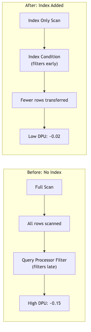
Figure 2: Before/After optimization comparison showing the impact of adding an index, with an 81% DPU reduction.

Cleanup

To avoid ongoing charges, remove the resources created during this walkthrough:

-- Drop indexes
DROP INDEX IF EXISTS idx_txn_date;
DROP INDEX IF EXISTS idx_txn_desc;
DROP INDEX IF EXISTS idx2;
DROP INDEX IF EXISTS idx1;
DROP INDEX IF EXISTS idx_account_customerid;
DROP INDEX IF EXISTS idx_transaction_customerid;

-- Drop tables
DROP TABLE IF EXISTS transaction;
DROP TABLE IF EXISTS account;
DROP TABLE IF EXISTS customer;

Then delete the Amazon Aurora DSQL cluster from your terminal. If deletion protection is enabled (the default), disable it first:

aws dsql update-cluster \
  --identifier <CLUSTER_ID> \
  --no-deletion-protection-enabled \
  --region <REGION>

aws dsql delete-cluster \
  --identifier <CLUSTER_ID> \
  --region <REGION>

Replace <CLUSTER_ID> and <REGION> with your values.

Conclusion

In this post, we showed how to use EXPLAIN plans to diagnose and optimize query performance in Amazon Aurora DSQL. The core principle: push filters as close to storage as possible. Index Conditions (Level 1) reduce data read at the index. Storage Filters (Level 2) reduce data transferred to compute. Query Processor Filters (Level 3) are the least efficient because all data has already moved across the network.

We demonstrated a consistent pattern: diagnose with EXPLAIN, identify filter placement, improve performance with targeted indexes, and validate with EXPLAIN ANALYZE VERBOSE to confirm DPU reduction. In our tests, adding an index to the transaction table reduced Total DPU from 3.39 to 0.66 (81 percent reduction), and adding an INCLUDE column to the account index removed the Storage Lookup entirely. For multi-table queries, redundant predicates and CTE late materialization provide additional levers to reduce unnecessary data movement.

To get started, try these next steps:

1. Run EXPLAIN on your top 10 most expensive queries. Identify which predicates are at Level 2 or Level 3, and prioritize index changes for the highest-DPU queries first.
2. Set up Amazon CloudWatch alarms for DPU thresholds. Monitor your DPU consumption over time and get alerted when queries exceed expected costs.
3. Review your index coverage. Look for Storage Lookup nodes in your most frequent queries and add INCLUDE columns where needed.

For more information, refer to Introducing Amazon Aurora DSQL, the Aurora DSQL EXPLAIN plans documentation, Amazon Aurora DSQL pricing for DPU cost context, and the Aurora DSQL User Guide.

About the authors