Build a genomics data lake on AWS using Amazon EMR (Part 1)

As data emerges from population genomics projects all over the world, researchers struggle to perform large-scale genomics analyses with data scattered across multiple data silos within their organizations. In order to be able to perform more sophisticated tertiary analysis on genomics and clinical data, researchers need to be able to access, aggregate, and query the data from a centralized data store in a secure and compliant manner. The Variant Call Format (VCF) is not an ideal way to store this data when it needs to be queried in a performant manner, so we need to convert it to an open format with efficient storage and performance.

Open, columnar formats like Parquet and ORC are more efficient at compression and perform better in the types of queries typically performed on genomic data. In this blog post, we build a post-secondary analysis pipeline that converts Variant Call Format files (VCFs) into these formats to populate a genomics data lake built on Amazon Simple Storage Service (Amazon S3). We use Hail, a genomics software tool from the Broad Institute, on Amazon EMR to perform the data transformation. In part 2 of this blog series, we will show how data can be interactively queried using Amazon Athena or Amazon Redshift and we discuss the benefits of using columnar formats and other optimizations to further improve query performance.

Solution overview

To demonstrate how to transform the data, we use the 1000 genomes DRAGEN re-analyzed dataset, which contains 3202 whole genome VCFs, from the AWS Registry of Open Data. The transformed data is available on the AWS Registry of Open Data at the following:

s3://aws-roda-hcls-datalake/thousandgenomes_dragen/

The following steps are involved in transforming VCFs to Parquet to prepare them for the data lake:

Store the raw VCFs (in .bgz or uncompressed form) in an S3 bucket.
Create an EMR cluster (with Hail installed).
The PySpark script that performs the transformations of the VCFs runs on the EMR cluster; the output Parquet files are written to an S3 bucket.
Convert annotations into Parquet using AWS and write them into an S3 bucket.
The Parquet data can then be crawled by an AWS Glue crawler and tables written to the AWS Glue Data Catalog, to be queried through Amazon Athena.

The high-level architecture of this process is shown in the following diagram:

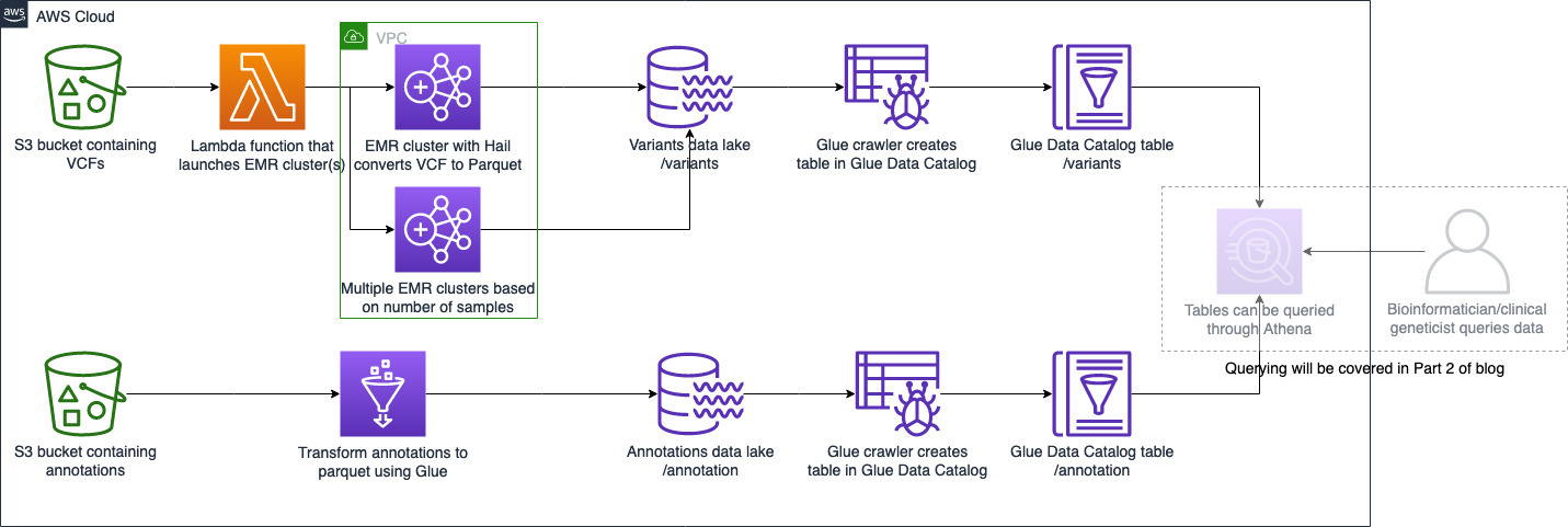
Figure 1: High level architecture diagram

Prerequisites

An AWS account with administrator permissions

Transforming a single VCF into Parquet

In this post, we use the 1000 genomes high coverage phase 3 data that was reanalyzed using Illumina DRAGEN 3.7. The source VCFs are available through the AWS Registry of Open data at the following:

s3://1000genomes-dragen/data/dragen-3.5.7b/hg38_altaware_nohla-cnv-anchored/

Each of the 3202 single sample VCFs contains approximately 5-6 million variants. We convert these VCFs into a flat table with all the fields retained, including all the info and format fields.

We use an EMR cluster with a custom AMI with Hail 0.2 compiled and configured. You can find more about how to set up Hail on Amazon EMR and explore genomic data using notebooks here. Hail can import VCFs in block compressed format (.bgz format) or uncompressed format. Since the 1000 Genomes DRAGEN-reanalyzed VCFs on the Registry of Open Data are block compressed, they need to be renamed from .gz to .bgz. The following Python code snippet uses Hail to convert the VCF into a Parquet table that is written to an S3 location.

import hail as hl
hl.init()
vds=hl.import_vcf(filename,reference_genome='GRCh38')
#flatten the Hail Matrix table
variant_table = vds.make_table()  
#convert to a Spark Data Frame   
vt_spark=variant_table.to_spark() 
#write Parquet file to S3 bucket
vt_spark.write.parquet(S3path)

The file name is the S3 path to the VCF file. You should specify the reference genome, since the default genome is GRCh37. Hail imports the VCF as a matrix table, which can then be converted into a Spark DataFrame. The sample script in the GitHub repository retains all the INFO and FORAT fields in the VCF and adds a column with the sample ID. We also create a field variant_id by joining the chromosome, position, Ref, and Alt fields, since this uniquely defines the variant. This DataFrame is then written out in Parquet format to an S3 bucket. Each sample is written out to a different S3 prefix, as in the following example:

s3://aws-roda-hcls-datalake/thousandgenomes_dragen/var_partby_samples/NA21144/

It is possible to perform custom transformations on the variant data using the Hail API to process multi-sample VCFs; to limit to variants in specific regions using a BED file; and to perform QC operations or annotate the variants using VEP. The following is an example of how to use a BED file to limit variants to regions of interest in a matrix table ‘vds’ that has been imported from a VCF file.

bed = hl.import_bed(bedfile,reference_genome='GRCh38')
filtered_variants = vds.filter_rows(hl.is_defined(bed[vds.locus]))

As in the previous example, once the Hail matrix table has been filtered or modified as required, it can be converted to a Spark DataFrame. Then, it can be written into an S3 bucket in a columnar, compressed format like Parquet. The advantages of using columnar formats like Parquet are explained in Part 2 of this blog series.

In the example script, each sample is written out to a different prefix under the output S3 bucket. This partitions the data by sample. Partitioning big datasets by a commonly used query filter is useful because the query engine can ignore irrelevant data and scan only a limited amount. Part 2 of the blog series explains how partitioning affects query performance.

Bulk transformation of a batch of VCFs

It is common to sequence and process genomics samples in batches. Batch processing of a large number of VCFs can be achieved either by running the batch as multiple Amazon EMR steps or by using multiple EMR clusters. In this example, we use multiple EMR clusters to simplify the automation of batch processing. However, it is possible to use a single cluster with significant custom performance tuning, in terms of steps concurrency and cluster memory, to process samples within a desired time. Due to the cluster provision time, starting up an EMR cluster to process a single sample is inefficient, so it is preferable to batch the new samples and process them in bulk. Each EMR cluster can be configured to process a given set of samples and automatically terminate on completion. This is subject to account service limits for EC2 instances that are launched by Amazon EMR.

To automate this process, you can have a regularly scheduled Lambda function process samples that are uploaded into a new prefix on an S3 bucket. You could also trigger the Lambda function based on S3 events, such as when a new file is uploaded into an S3 bucket.

To simplify the conversion of a large number of samples, we provide an AWS CloudFormation template. The template processes samples quickly by requesting multiple EMR clusters and distributing samples to each.

How to use the provided solution

To deploy the necessary resources into your AWS resources, launch the CloudFormation stack using template here or launch directly. This template has some mandatory fields and some optional fields. The optional fields provide flexibility to give your own configurations to the solution. Use the following steps to deploy the solution:

Enter the parameters shown in the table below. The table’s Required? column specifies whether parameters are required or optional.

*The default value for the number of samples processed per cluster is 100, based on some benchmarking using two r5.xlarge core nodes and one r5.xlarge task node, which took approximately 1 minute per whole genome sample in the 1000 Genomes dataset. This can be adjusted up or down based on the desired sample processing time and EMR cluster configuration.

2. After all the CloudFormation parameters are filled in, choose Next.

3. On the next screen, leave all the sections as default and choose Next again.

4. Review the parameters passed, select the two boxes on the bottom, and choose Create Stack.

Once the CloudFormation deployment completes, the following two resources are created:

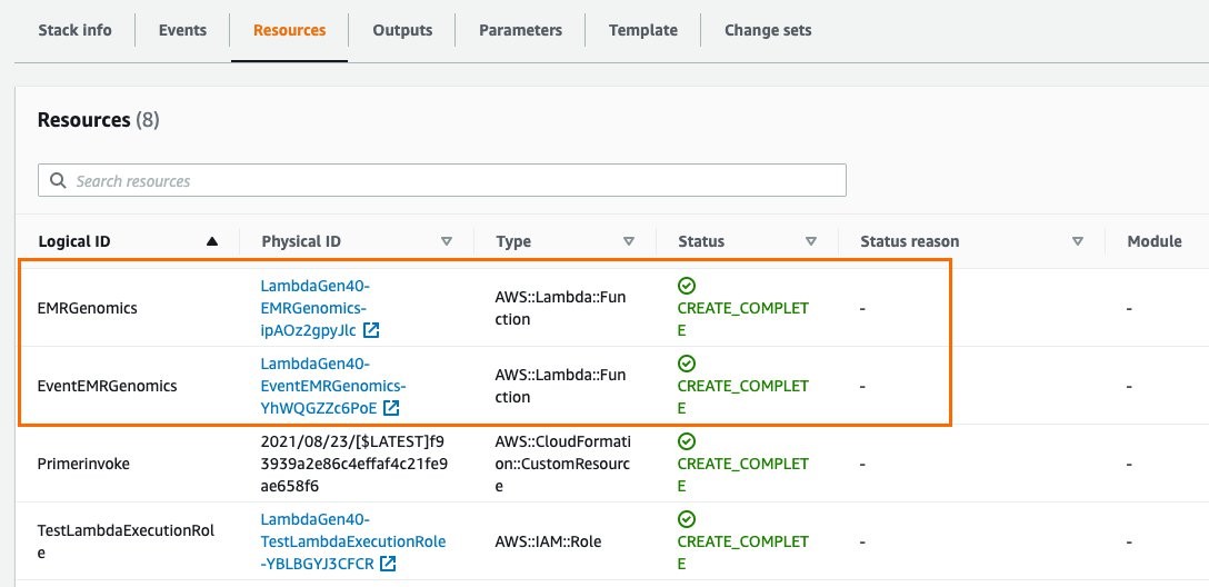
Figure 2: Resources created by the Cloudformation template

EMRGenomics Lambda function: This Lambda function is automatically triggered as soon as it is created, launching the required number of EMR clusters (with Hail installed). The number of clusters depends on the total number of samples (VCF files in .bgz or uncompressed format) in the input S3 bucket and on the “Number of samples per EMR cluster” parameter. For example, the default parameter is 100 samples per EMR cluster. Using the default parameter, if there are 500 samples in the input S3 bucket, five EMR clusters would launch and each would process 100 samples.
EventEMRGenomics Lambda function: This Lambda function is created by the stack, but it is not triggered during the initial run. It is meant to be triggered by an S3 event notification for automating the pre-processing of sample files on an ongoing basis. If new samples are uploaded to an S3 bucket that has event notification set up, it can be configured to trigger the EventEMRGenomics Lambda function. This lambda function would launch the EMR clusters (with the same configuration, PySpark script, and output S3 path configured through the CloudFormation template). EMR clusters would then perform the same transformation of VCF files to Parquet using the PySpark script.

To set up the event notification for your S3 bucket, follow the step-by-step guide here. In step 7a, for destination type, select Lambda Function. In step 7b, choose EventEMRGenomics.

Annotation data

Genomic analysis requires detailed annotations of variants. Annotations may include gene name (if variant is in a coding region), variant type (nonsense, missense, splice, intronic, intergenic, and so on), the effect of the variant on the protein, and the potential clinical significance of the variant (if known), to name only a few. These annotations can come from multiple sources. Some commonly used, publicly available annotation databases are ClinVar, dbSNP, dbNSFP, and gnomAD. Each database is updated at different frequencies. For example, ClinVar is updated weekly while gnomAD is updated much less frequently.

The traditional method—adding annotations to VCFs using tools like VEP, Annovar, or snpEff—has the advantage of keeping all the information within the VCF, which can then be converted into Parquet. However, when any annotation source is updated, the VCF and the Parquet files would need to be regenerated. A more efficient method is to maintain annotations separately and update them as needed. This requires a separate process to convert the annotations into a data lake-ready format like Parquet. We recommend using AWS Glue to transform the annotation data into Parquet. Then add the tables into the Data Catalog as detailed here or use Athena as shown in the following code:

create table annotations_Parquet
  with (
    format = 'Parquet',
    partitioned_by = array['chrom'],
    external_location = 's3://<Your_s3_bucket>/annotations_Parquet/'
    )
as select *, chr as chrom from genomics_datalake.raw_annotations;

Query data

Once the variant data has been converted to Parquet, create an AWS Glue crawler to crawl the data by pointing it to the S3 location that contains the Parquet files. Step-by-step instructions for creating an AWS Glue crawler can be found at this link. You can deploy this template to create tables for the 1000 Genomes DRAGEN dataset that is available in the AWS Registry of Open Data.

The Parquet-transformed 1000 genomes data that is partitioned by samples is available on the AWS Registry of Open Data at this link. ClinVar and gnomAD are also available in data lake-ready formats in the AWS Registry of Open Data. See how to add them to your Data Catalog at this github repository. They can then be queried using Amazon Athena. We dive deeper into how to query the data and optimize query performance in part 2 of this blog series.

Cost and performance considerations

An EMR cluster consists of a master node, core nodes, and task nodes. The instance type of the task nodes and the number of nodes depends on the volume of the input data. For the 1000 Genomes 30x whole genome VCFs, we used m5.xlarge master node and 2 r4.8xlarge core nodes to process 100 VCFs per EMR cluster. Typically, it takes approximately 10-15 minutes to prepare an EMR cluster.

The time required to process each sample varies based on the size of the VCF and the cluster resources. In the 1000 Genomes example, the average processing time per sample was approximately 60 seconds. Since we were processing a large number (3202) of samples and wanted the processing to complete within a reasonable amount of time, we used 35 clusters and configured each cluster to process approximately 100 samples. Processing all the samples took just over two hours, but this can vary significantly based on the actual samples processed.

Cleanup

The EMR clusters that are created as part of this CloudFormation template are set up to terminate automatically once the processing is done, so there is no additional cleanup required.

Conclusion

In this blog post, we transform genomic data into a compressed, columnar format that can be ingested into a genomics data lake for efficient analyses. This can help break data silos, mitigate the problem of multiple people with separate copies of a dataset, and help individual researchers with data management. Organizations can consolidate data and apply uniform governance and security policies on their datasets, and individuals can focus on scientific questions.

Our solution can be used in conjunction with others that use AWS Lake Formation for access control. For instance, it can be used with this post addressing multi-account access or with this post on using tags to manage resources and access.

In part 2 of this blog series, we will show how data can be interactively queried using Amazon Athena or Amazon Redshift and we discuss the benefits of using columnar formats and other optimizations to further improve query performance.

For more information on Amazon services in Healthcare, life sciences, and genomics, please visit aws.amazon.com/health.

________________________________________________

AWS for Industries