AWS for Industries
Machine Learning Leukemia diagnosis at Munich Leukemia Lab with Amazon SageMaker
Munich Leukemia Lab (MLL) is a leading global institution for leukemia diagnostics and research, operating within a highly innovative environment. MLL aims to shape the future of hematological diagnostics and therapy through state-of-the-art molecular and computational methodologies. To this end, MLL partnered with the Amazon Machine Learning Solutions Lab (MLSL) and Mission Solutions Team (MST) to create an automatic leukemia diagnosis pipeline leveraging machine learning and the knowledge of subject matter experts at MLL.
In this post, we detail our collaboration in creating a robust ML model using Amazon SageMaker to detect 30 different leukemia subtypes using only next generation sequencing (NGS) data. We provide insights on:
- Handling NGS variant call files to generate useful features for classification
- Exploring separability of the different classes based on similarity metrics
- Finding the best model for leukemia subtype classification and interpretability
- Takeaways from the collaboration
Introduction
Leukemia refers to a group of blood cancers that present a substantial healthcare challenge, causing over 310,000 deaths annually worldwide, according to the 2018 Global Burden of Disease study. Diagnosis and treatment are highly challenging due to heterogeneity; there are 31 leukemia entities (subtypes) defined by the World Health Organization as of 2017.
Currently, leukemia is diagnosed using a combination of methods. These methods require complex equipment and highly skilled clinical laboratory scientists and technicians – scarce resources – which increases turnaround times as well as costs. Average times from sample receipt to reporting can take up to ten days.
A paradigm shift in diagnostic methodology
Next-generation sequencing (NGS), a massively parallel DNA sequencing technology that is able to read an entire human genome within a day, has shown great promise for identifying leukemia subtypes as well as prescribing more targeted and effective treatment.
Prof. Dr. Torsten Haferlach, CEO of MLL, said, “To establish this paradigm shift, from a primarily manual review of morphological features by experienced experts, to an objective, algorithmic approach using molecular genetics-based features, MLL partnered with the Amazon ML Solutions Lab to tackle this extraordinary feat. This work will lead to more cure and prolonged life time of all patients.”
Cancer classification based on NGS data using machine learning
The Amazon Machine Learning Solutions Lab took on the challenge of assisting MLL in developing an innovative clinical decision support model based on a next generation sequencing (NGS) dataset. NGS data are extremely high dimensional, and are usually comprised of very small amounts of quality training data. MLL, having completed the 5,000 genomes project, has one of the largest datasets in this domain. The majority of samples from the 5,000 leukemia patients involved were sequenced using whole genome sequencing (WGS) and whole transcriptome sequencing (WTS), and diagnosed using WHO gold standard orthogonal diagnostic methods.
Data preparation
With the global scope of MLL’s research, it is imperative that data is kept in cloud services that are secure and compliant with privacy regulations. AWS is available in many countries and regions, which provides convenience and low cost for customers. All customer data can be stored and accessed in any region within AWS. In this particular case, the data from MLL was stored in Amazon S3 buckets within the customer’s selected region in Frankfurt to meet requirements for healthcare data.
NGS data from DNA (whole genome sequencing) and RNA (whole transcriptome sequencing) was initially processed by MLL using a custom pipeline. From WGS, there are several types of variants that are extracted: single nucleotide variant (SNV), structural variants (SV) and copy number variants (CNV). The SV and CNV data are in VCF files, which have a complex structure. VCF files include variant call information like the chromosome and segment location of the variant, the read coverage and the variant filtering criteria. VCF files for the SV and CNV data cannot be easily imported into a format that can be ingested by machine learning models. Further processing is needed to extract and aggregate features based on the chosen granularity level, which could be at the level of genes, chromosome bands or chromosomes.
From the WTS pipeline, gene expression (GE) and gene fusion (GF) data can be obtained. The advantage of GE data is that it already has a tabular format where each row is a patient and each column is the expression value of a gene, so there are no further transformations and only a quick normalization procedure that must be carried out. GF is more similar to the files obtain for WGS, so similar transformations are performed.
We established a pipeline that takes the data files from each patient and transforms them into a vector of features from each modality. For SV files, we extracted five types of variants: insertions, deletions, duplications, translocations, and inversions on the gene level for short segments. For longer segments, we extracted features based on the band or chromosome level. This approach was also used for CNV files. For WTS data, gene expression is extracted in the form of read counts and is normalized following the normalization weighted trimmed mean of M-values (TMM) method. As a result, we generated more than 70,000 features from the five original tables (SNV, SV, CNV, gene expression, gene fusion). Missing data was imputed differently depending on the source type. For some types, we used the lowest value (CNV) or zero (SNV, SV, gene expression). At the end of the data processing, each patient possesses the same number of features, which can be used as the input for a machine learning model.
We evaluated several strategies to combine these different modalities, including stacking or ensembling models trained on each individual modality. However, separately handling these data types does not take into account the observation that there are nonlinear interactions between features of different modalities (e.g., connections between copy number amplification/deletion and gene expression level up- or down regulation, SVs associated with aberrant gene expression). The model has to be able to account for such interactions to perform well, which is why concatenating all feature types to allow the model to learn interactions between them led to the highest predictive accuracy.

Figure 1: Overview of the files that were processed to get a tabular dataset for training. “||” refers to concatenation of the vectors obtained for each file type.
Pre model analysis
The dataset from MLL contains patients with 30 different leukemia subtypes. Some of the subtypes are far more frequent than others, resulting in a highly imbalanced dataset.
 Figure 2: Number of patients by leukemia subtype.
With all the different types of data converted to tabular format, we started a feature engineering process that involved collaboration with experts from MLL. They surveyed the literature to find important biomarkers associated with each leukemia subtype. With this in mind, we designed a process to aggregate and combine the original features into biomarkers.
The final dataset had about 4500 rows representing patients and 800 columns containing the extracted biomarker data, combined with other important features for each data type (CNV, SNV, SV, etc.) outside of the original biomarker feature set. In other words, each patient’s genome and transcriptome was represented by a vector with 800 entries.
Among the 30 leukemia subtypes, some of them are closer to each other than to the rest. For example, MPAL, AML, and BCP-ALL are very similar; sometimes, the genetic profile from a patient with MPAL might be more similar to a patient with BCP-ALL than to another patient with MPAL. This presents a challenge for both the machine learning algorithm and human experts to differentiate them. To investigate how similar leukemia subtypes were among each other, we calculated the distances between every patient and the rest of the samples and recorded which were the closest two neighbors. Then, we aggregated the neighbors by leukemia subtype and found that indeed, in some of the classes, less than 20% of the patients in that subtype are very similar to each other. This is shown in Figure 3. If we find the MPAL circle, we can see that only 13% of all the patients with MPAL are similar to each other, and that the majority of similar patients belong to AML and BCP-ALL.
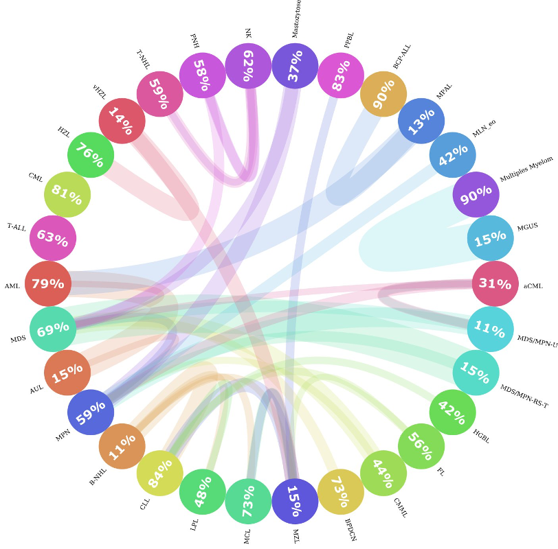
Figure 3: Entity Similarity Circos plot. This figure shows how similar leukemia subtypes are to each other. Each circle represents a leukemia subtype and the number inside the circle captures the percentage of neighbors that are of the same subtype. If there is a significant portion (>= 10%) of patients that are more similar to patients from another entity, then a connection is drawn (colored line) from one entity to the other. The thickness of the line represents how big the portion of patients were similar to other groups. The color of the line represents the direction of the connection, i.e., patients from one entity belonging to other groups; is represented with the color of the original entity. For instance, Patients from the MGUS class were more similar to patients with Multiple Myeloma. But there are no significant connections the other way around.
Modeling
To predict patient leukemia subtypes, we trained a multi-class classifier. With the classifier and the feature extraction pipeline, we prototyped a system that automatically determines patient leukemia subtype based on WGS and WTS data using Amazon SageMaker Notebooks. Amazon SageMaker is a cloud machine learning platform that can be used to build, train, and deploy models for virtually any use case. Notebook instances provide flexible environments to build machine learning models, saving users time and effort from managing the underlying compute infrastructure.
We used LightGBM, a gradient boosting algorithm, to build our first classifier. We also used SageMaker Hyperparameter Optimization (HPO) jobs to tune our model’s hyperparameters, an approach that automatically finds the optimal configuration of any algorithm without manual effort by using Bayesian optimization. Using HPO, our LGBM model performance reached an accuracy of 82% on 5-fold cross-validation. For some entities with unique biomarkers, the accuracy is very high. CML has an almost unique fusion gene BCR-ABL as a biomarker, and the LGBM model reaches 97% accuracy for CML.
However, for entities with very few patients, with a strong similarity to other entities or those which require an extra laboratory analysis during traditional diagnosis, the model does not perform as well. For dealing with small and imbalanced samples, you can use the generation of synthetic data. We tried different methods including LoRAS and ADASYN, but did not see any model improvements.
Models that utilize few-shot learning have also been used for classification problems with very few samples for a category. We implemented a few-shot learning architecture for disease type prediction, but did not see any improvement. This is likely due to the challenge of learning the distribution of a leukemia type with the very small number of patients we had available for each type.
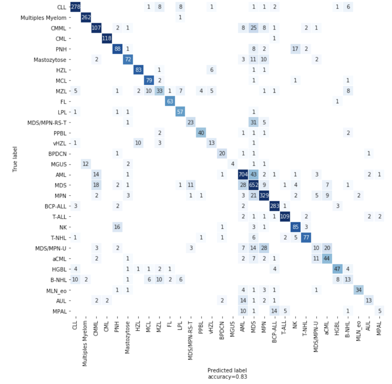
Figure 4: Confusion matrix showing the number of correct and incorrect predictions from the model
Explanation
When a machine learning model is used to make a prediction, an understanding of why the prediction was made is as important to MLL researchers as the prediction itself. In order to understand why the model is making particular predictions, we leveraged the SHAP python library. With this library, we can analyze a prediction from the trained model and gain insight into the features used to make the classification. We applied SHAP to our LGBM model and analyzed feature impacts at both the sample level and the global level. Figure 5 illustrates an application of SHAP at the patient level for two individuals diagnosed with CML compared to CML correctly predicted cohort. By using a decision plot, we can observe which features are the most important contributors to the model’s prediction.

Figure 5: SHAP force plot for a CML patient predicted correctly, and a decision plot for every patient with CML, 117 predicted correctly (yellow lines) and one predicted incorrectly (red line). The features are shown on the y-axis in order of mean importance for all patients with CML; note the well-known BCR/ABL1 features at the top. These features pushed the classifier toward CML for both patients, but for the patient that was predicted incorrectly, the gene expression features caused the classifier to predict that the patient had BCP-ALL. These decision plots are useful to understand how much each feature contributes to the classification; note the x-axis is ‘log-odds’, so a feature that pushes the output from 0 to 10 is many orders of magnitude more important than a feature that pushes the output from -5 to 0.
Takeaways and outlook
Collaboration with domain experts: This has been crucial, and will remain a key part of the application of machine learning and AI in the medical domain. In addition to sharing the largest and highest quality dataset of its kind, MLL facilitated the creation of the machine learning model by contributing their substantial domain expertise every step along the way. In the beginning of the project, we coded our feature space on the gene level and we only achieved an accuracy of 67% on 30 leukemia subtype predictions. By using MLL’s manually curated biomarkers and genetic features – feeding the model what is already known about this domain by human experts – we achieved 77% accuracy. Later, we added more features into the feature space and further increased model performance by 5%.
Using the right tooling: Working with SageMaker significantly accelerated this project. Because SageMaker is a fully managed platform and integrated for ML, it allowed the team to focus on the data science work without having to worry about managing infrastructure. The built-in automatic model tuning feature increased the accuracy of the model without having to manually tune the model architecture or hyperparameters, saving time and optimizing the model.
Interpretability and explain-ability: MLL continues innovating and improving their approach, and working on their vision towards lightning fast, highly accurate, and algorithmically objective leukemia diagnosis benefiting patients worldwide. In the words of Benjamin Bell, quoted by Prof. Haferlach during a keynote talk: “…AI will not replace doctors, but instead will augment them, enabling physicians to practice better medicine with greater accuracy and increased efficiency.”
Conclusion
MLL’s mission is to improve the care of patients with leukemia and lymphoma through cutting-edge diagnostics. To do this, the lab uses an interdisciplinary approach combining six disciplines – cytomorphology, immunophenotyping, chromosome analysis, fluorescence in situ hybridization (FISH), molecular genetics, and bioinformatics – resulting in one comprehensive integrated laboratory report.
“In general, we can distinguish disease subtypes through phenotypic methods like cytomorphology, immunophenotyping, and genetic techniques. In the future, molecular techniques will be the most important methods in helping us capture all this information,” said Prof. Haferlach. “Today, genetic diagnostics relies on cytogenetics and mutation analysis. Soon, we will be doing whole-genome and whole-transcriptome sequencing.”
Whole-genome sequencing can identify more structural variants and copy number changes than are evaluable through chromosome analysis, and it can also be used for mutation detection and analysis, he explained. “There could be one assay that does everything,” he predicted. “If we also include gene-expression profiling in our diagnostics, we can even catch features that are now determined by immunophenotyping and cytomorphology. This is our vision for the future.”
“We are professors and researchers,” Dr. T. Haferlach echoed. “We want to always be on the cutting edge of what is next.” That desire has pushed the MLL founders to fully embrace and incorporate technology into their lab and collaborate with AWS to achieve innovation.
To learn more about genomics in the AWS Cloud, see aws.amazon.com/health/genomics.