AWS Web3 Blog
Optimize tick-to-trade latency for digital assets exchanges and trading platforms on AWS: Part 2
Part 1 of this series covers the high-level architecture of a Centralized Exchange (CEX) and Market Maker (MM) and networking integration patterns. This post builds on that foundation by focusing on EC2 compute optimization. In this post you will learn how to
- Reduce tail latency by up to 29% at p99.9 by selecting the right EC2 instance size and using bare metal instances to eliminate hypervisor jitter.
- Prioritize optimizations in the correct order using a five-tier latency hierarchy, from regional placement (millisecond impact) down to OS tuning (microsecond impact).
- Establish reproducible baselines and measure each change using the trading-latency-benchmark tool, an open source solution that pairs simulated trading clients against a mock matching engine on EC2.
Market Maker Trading Hot-Path
Market makers (MM) provide continuous buy and sell quotes for financial instruments. They profit from the bid-ask spread while absorbing inventory risk. MM compete on spread tightness, execution speed, and pricing model sophistication. Market making is highly competitive. Key challenges include adverse selection (trading against better-informed counterparties), managing exposure in volatile markets, and the compounding cost and complexity of a relentless latency arms race. They deploy strategies at high order rates with microsecond-level execution. We use terms HFT and MM in this post interchangeably.
Tick-To-Trade
Tick-to-trade measures the latency of your trading hot-path. You measure it from where the exchange acknowledges a message in its order gateway, resulting in market data update (tick) to when your software transmits an instruction (order, cancel, replace, etc.) back to the exchange, as shown in Figure 1.
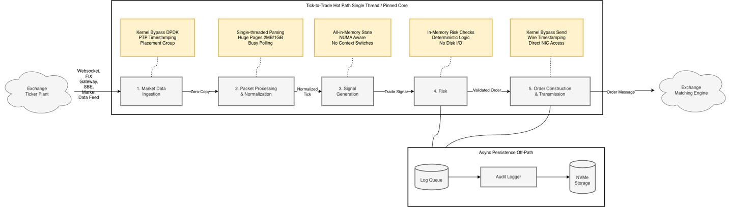
Figure 1: Market Maker Trading Hot-Path
The following table calls out the critical aspects about each of the 5 processing stages depicted in Figure 1:
| Stage | Description | Critical Compute Requirements |
| 1. Market Data Ingestion | Tick arrives at EC2 from exchange | Placement close to market data gateway; fine-grained, ideally nanosecond timestamps by using hardware receive timestamps to separate network vs. processing bottlenecks |
| 2. Packet Processing & Normalization | Raw packets parsed, validated, normalized | High clock speed for single-threaded parsing; large L1/L2 cache for sequential event stream processing |
| 3. Signal Generation | Algorithms analyze data for buy/sell signals | Sufficient RAM to hold algorithm state entirely in-memory without paging |
| 4. Risk Check | Pre-trade validation of limits, exposure, compliance | In-memory risk profiles and reference data; async logging to NVMe to isolate storage latency from critical path |
| 5. Order Transmission | Order formatted and sent to exchange | Placement close to matching engine to reduce propagation delay and race conditions |
Table 1: Market Maker Trading Hot-Path Stages
Understanding compute latency optimization
On the surface, you follow the same general steps in every trading strategy: decode incoming market data, generate trading signals, and execute them. However, your proprietary software stack, trading style, and exchange environments create optimization criteria unique to your firm. AWS shared networking infrastructure differs from purpose-built on-premises environments designed solely for trading. As a result, you should approach instance selection and network-level variability as a statistical optimization problem rather than a deterministic engineering exercise. Your goal is not to eliminate variance entirely. It is to deliver a consistent, measurable edge in execution quality. Regional placement, network path, OS configuration, and processor characteristics each directly affect your fill rates, execution quality, and trading economics. Effective optimization requires two foundational concepts.
- A hierarchy of latency impact that establishes the correct order of operations.
- Reproducible test environments that let you isolate and quantify each variable.
Hierarchy of Latency Impacts
Figure 2 presents a five-tier hierarchy. Each tier governs a distinct order-of-magnitude window of latency. Geographic placement and networking path optimization (1 ms to 100 ms) occupy the top tiers. Operating system and application micro-optimizations (1 ns to 5 µs) occupy the bottom. Upper tiers dominate your mean latency. Middle tiers (network path, instance selection) dominate your tail behavior. Optimizing in the wrong order is the most common and costly mistake in latency engineering. No amount of cache-line alignment or lock-free queue tuning recovers the milliseconds you lose by deploying in the wrong Region or routing traffic through an unnecessary network hop. The cost is concrete. Your adverse selection increases, your queue priority erodes, and your strategy becomes unprofitable before you reach the layers that would otherwise matter. In HFT, latency is a competitive metric, not just a performance one. Being microseconds slower than a competitor means you systematically receive stale fills, lose queue priority, and get adversely selected on every quote until your edge is consumed.
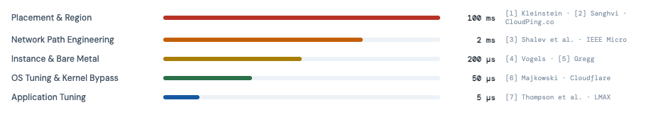
Figure 2: Hierarchy of Latency Impact
References:
- Kleinstein, D. “Measuring Latencies Between AWS Availability Zones.” Bits and Cloud, October 2023. https://www.bitsand.cloud/posts/cross-az-latencies
- Sanghvi, P. “Building a High Performance Trading System in the Cloud.” Proof Trading / Medium, January 2022. https://medium.com/prooftrading/building-a-high-performance-trading-system-in-the-cloud-341db21be100
- Shalev, L. et al. “A Cloud-Optimized Transport Protocol for Elastic and Scalable HPC.” IEEE Micro, Vol. 40, No. 6, pp. 67–74, November–December 2020. https://assets.amazon.science/a6/34/41496f64421faafa1cbe301c007c/a-cloud-optimized-transport-protocol-for-elastic-and-scalable-hpc.pdf
- Vogels, W. “Reinventing Virtualization with the AWS Nitro System.” All Things Distributed, September 2020. https://www.allthingsdistributed.com/2020/09/reinventing-virtualization-with-nitro.html
- Gregg, B. “AWS EC2 Virtualization 2017: Introducing Nitro.” brendangregg.com, November 2017. https://www.brendangregg.com/blog/2017-11-29/aws-ec2-virtualization-2017.html
- Majkowski, M. “How to Achieve Low Latency with 10Gbps Ethernet.” Cloudflare Blog, June 2015. https://blog.cloudflare.com/how-to-achieve-low-latency/
- Thompson, M. et al. “Disruptor: High Performance Alternative to Bounded Queues for Exchanging Data Between Concurrent Threads.” LMAX Exchange, 2011. https://lmax-exchange.github.io/disruptor/disruptor.html
Trading-Latency-Benchmark
To establish baselines and measure each optimization’s impact, you need a reproducible test environment. The authors of this post created trading-latency-benchmark, an open source tool that measures round-trip network latency for simulated trading workloads on EC2. The workflow follows three steps:
- Run the trading-latency-benchmark tool to establish a baseline.
- Apply optimizations from the hierarchy described in this post.
- Retest to quantify the impact of each change.
The tool pairs HFT client implementations (Java, Rust, C++) against a mock matching engine. It captures full latency distributions using HDR Histograms (a high dynamic range histogram data structure for recording and analyzing value distributions) up to p99.9. You can provision test environments spanning different EC2 instance types, networking configurations, and kernel parameters automatically. This makes it straightforward to quantify each variable in isolation.
The EC2-related latency numbers in this post use Single Instance Deployment loopback mode. A single EC2 instance runs both a C++ trading client and a Rust mock exchange server, communicating through the local loopback interface. You can reproduce these results in your own AWS account.
Optimizing Along the Latency Hierarchy
With the latency hierarchy and measurement tooling established, the following sections walk through each optimization layer top-down. You start with placement decisions that dominate overall latency and progress down to OS-level tuning that reduces jitter. Part 3 of this series covers kernel bypass and application-level tuning.
Placement – Region and Availability Zone (AZ)
Regional instance placement is the single largest contributor to overall latency. Deploy your market data ingestion workloads (see Figure 1) in the same AWS Region and same Availability Zone (AZ) as the CEX market data or order gateway. This reduces latency compared to deploying across Regions and Availability Zones.
For hybrid networking scenarios (on-premises to cloud), you can use AWS Direct Connect (DX) with dedicated low-latency connections such as dark fiber from AWS Direct Connect Partners.
Network Path Engineering
Within the same Region and same Availability Zone, evaluate latency-optimized and jitter-optimized connectivity options with your exchange partner. Jitter is the variation in latency between successive packets. The lower your jitter, the more predictable your execution timing.
- Cluster Placement Group (CPG) with Amazon Virtual Private Cloud (VPC-Peering) – lowest latency. Instances are physically co-located.
- VPC Peering – low latency. Direct routing between VPCs without middleboxes, especially useful establishing low latency connectivity between two AZs.
- AWS PrivateLink – secure, service-level connectivity. Exposes a specific service (not the full VPC) to consumers across accounts via NLB-backed endpoints. Scales to thousands of consumers with no CIDR overlap concerns.
Keep hot-path traffic point-to-point between instances. Avoid Elastic Load Balancing (ELB), AWS Transit Gateway (TGW), network address translation (NAT) routers, or inspection appliances on the critical path. For inter-VPC traffic, use VPC Peering as the lowest latency logical connectivity option. Consider requesting shared Cluster Placement Groups when co-locating with exchange infrastructure. For details and test results, see the One Trading and AWS: Cloud-native colocation for crypto trading blog post. A single Availability Zone can span multiple data centers and network spines. Placement optimization has two ordered priorities. First, minimize physical distance between instances. Second, minimize the number of congested network pathways your packets traverse.
To achieve this, use a practice called “EC2 hunting.” You launch multiple EC2 instances, each in its own Cluster Placement Group. You then run latency pings from each instance to a target endpoint and compare results across clusters to identify which instances deliver the lowest latency. You retain only the top-performing instances and their Cluster Placement Groups for your trading workloads. The trading-latency-benchmark tool automates this process. It handles instance provisioning with CPGs, distributed latency testing, and result reporting using Ansible playbooks. For a step-by-step walkthrough, see Latency Hunting Deployment Strategy.
EC2 Instance Selection
To choose the right instance type and size for your workload, evaluate compute performance, regional availability, and feature-availability.
Instance Size Selection
Select the largest instance size within a family to get exclusive access to the underlying physical host (full slot). This reduces CPU jitter from noisy neighbors. Bare metal instances (.metal) guarantee single tenancy and full P-state control. For general compute workloads, the Nitro hypervisor overhead is minimal. See Bare metal performance with the AWS Nitro System for details. For network-latency-sensitive trading workloads, however, the metal advantage is more pronounced. The following table shows results from the trading-latency-benchmark loopback performance test. The test compared .metal instances against their corresponding largest full-slot EC2 instance by simulating limit and cancel orders, then measuring round-trip times over the loopback address after OS tuning.
| Instance Family | Metal (p50) | Full-Slot (p50) | p50 Δ | Metal (p99.9) | Full-Slot (p99.9) | p99.9 Δ |
| m8azn | 17.7µs | 18.9µs | 6% | 19.4µs | 22.7µs | 15% |
| m5zn | 20.3µs | 23.6µs | 14% | 22.2µs | 31.0µs | 28% |
| C7i (24xl) | 20.3µs | 21.7µs | 6% | 22.0µs | 30.9µs | 29% |
Table 2: EC2 Metal compared with Full-Slot Instances
Median latency improvements range from 1.2µs to 3.3µs (6-14%). The tail latency advantage of metal instances is larger: 3.3µs to 10.9µs (15-29%) at p99.9. This gap at p99.9 is consistent with metal eliminating hypervisor scheduling jitter and noisy-neighbor interference, which primarily manifests in tail latency. If your tail latency directly impacts your fill rates and adverse selection risk, the metal instance advantage is material. Choosing the right EC2 instance type goes beyond raw compute performance.
For low-latency environments, you also need high-precision time synchronization, networking optimizations with high throughput, and low-latency storage.
Time Synchronization
As described in the tick-to-trade process flow (Figure 1), you need precision time for timestamping, cross-system correlation, and regulatory compliance.
With the Amazon Time Sync Service, you get three complementary capabilities at no additional charge.
- Network Time Protocol (NTP), available on all EC2 instances. Clock error bound is typically under 100 microseconds.
- Precision Time Protocol (PTP) Hardware Clock (PHC) on supported instances . This tightens the error bound to typically under 40 microseconds.
- Hardware packet timestamping, which attaches a 64-bit nanosecond-precision timestamp to every incoming network packet at the Nitro NIC level.
These capabilities let you attribute latency precisely across each segment of your tick-to-trade path. Note that hardware timestamps require traffic to traverse a physical network interface. In local loopback tests, packets stay within the kernel’s network stack, so no PHC timestamp is attached. For more details on PTP measurements and clock error bounds, see It’s About Time: Microsecond-Accurate Clocks on Amazon EC2 Instances. For setup instructions, see the PTP quick start guide.
Networking
Network-optimized instances with enhanced networking (for example, m6in, c6in, m8azn) can reduce your tail latency by up to 85% at p99.9 and increase single-flow bandwidth by 5x. Your Elastic Network Adapter (ENA) driver version and configuration directly affect packet processing performance. Use the latest ENA driver and follow the ENA Linux Driver Best Practices Guide for tuning recommendations.
ENA Express uses AWS Scalable Reliable Datagram (SRD) transport to reduce p99/p99.9 tail latency for instance-to-instance traffic within a placement group. However, for HFT workloads ENA Express is rarely the right choice. SRD shifts more processing to the driver, increasing CPU overhead per packet. It can modestly inflate your p50 baseline latency. It also requires both endpoints to have ENA Express enabled. Where p50 consistency matters as much as tail reduction, use conventional ENA with kernel bypass techniques such as the Data Plane Development Kit (DPDK), Express Data Path (XDP) zero-copy, or Single Root I/O Virtualization (SR-IOV). See the networking_benchmarks for DPDK and XDP zero-copy sample implementations using ENA.
Storage Considerations
Instance store block storage for EC2 instances offers sub-millisecond latency but is ephemeral. Use it for temporary data such as caching or high-speed processing tasks where you do not need persistence. See the list of instances that support instance store.
For persistent storage, Amazon Elastic Block Store (EBS) supports databases and transactional systems that require durability. You can attach EBS volumes to all your EC2 instances. Provisioned IOPS SSD (io2) Block Express volumes deliver high IOPS and throughput, making them competitive with instance-store in many scenarios.
Operating System
The next optimization layer is the operating system (OS), typically Linux in latency-critical environments. Your kernel version significantly impacts performance. Linux kernels 6.1+ deliver measurably lower latency for trading workloads.
Ubuntu with kernel 6.12+ is the preferred distribution for latency-sensitive trading, followed by Rocky Linux and Red Hat Enterprise Linux. Amazon Linux is less commonly used for these workloads because its default configuration and kernel options prioritize general-purpose compatibility over latency optimization. ENA drivers compile across supported distributions when prerequisites are met. During performance tuning, you typically disable default management packages such as AWS Systems Manager (SSM) and Amazon CloudWatch to minimize overhead.
Linux Kernel and OS Optimization on EC2
Linux kernel tuning reduces latency and jitter by making CPU scheduling, power management, interrupt request (IRQ) placement, non-uniform memory access (NUMA) locality, and network-stack parameters more deterministic. Your goal is to verify that critical trading threads run predictably, without interruption from kernel housekeeping tasks.
The trading-latency-benchmark repository includes a comprehensive Ansible playbook (tune_os.yaml) that automates these optimizations. See the OS Tuning Reference for a complete overview of tunables.
OS Tuning Impact on Loopback Latency
To quantify the impact of kernel and OS tuning, the authors ran the trading-latency-benchmark loopback test before and after applying tune_os.yaml across multiple instance types and sizes. See the OS Tuning Benchmark Results for the raw measurements.
Tail latency improves almost universally. Even where median barely changes (m8azn.metal: 1% p50 improvement), max latency dropped 27%. The tuning helps mitigate jitter sources such as IRQ interference, kernel thread scheduling on application cores, and C-state transitions, rather than improving steady-state throughput. Tuning impact varies by instance type. Intel c7i and previous-generation AMD m5zn benefit most (28-36% p50 improvement). Newer m8azn and Graviton c8g show minimal median gains, which suggests they already operate closer to their floor out of the box. Graviton c8g shows remarkable consistency. While not the fastest in absolute terms (21.4 µs p50), its latency distribution is extremely tight before and after tuning. This reflects Graviton’s architectural simplicity. No hyper-threading, no complex C-state/P-state management.
Conclusion
Cloud-based latency optimization is a multi-dimensional problem. Key takeaways from this post.
Optimize the right order. A perfectly tuned kernel cannot compensate for a suboptimal Region selection. Follow the hierarchy from placement through OS tuning.
Test iteratively. Performance varies across instance types, generations, and architectures. No single configuration is universally the best. Results shift with new instance families, firmware updates, and application changes. The trading-latency-benchmark tool lets you run these tests against your own workloads with reproducible results.
Metal matters for tail latency. Median differences are modest (6–14%), but p99.9 diverges 15–29% in favor of metal instances. If your tail latency impacts fill rates and adverse selection, the metal advantage is material.
Graviton for consistency. The c8g.metal shows tight distributions (21.4µs p50, 23.4µs p99.9), reflecting Graviton’s architectural advantages. If your stack targets ARM64, c8g offers strong price-performance with minimal tuning.
Instance selection is a trade-off between raw latency and features like PTP and instance store.
In Part 3, we’ll cover hybrid deployment with Direct Connect, multicast strategies, and kernel bypass techniques including AF_XDP and DPDK.
Now go clone the trading-latency-benchmark repository, customize it for your needs, and use it as a reproducible latency test environment in your own AWS account!