Building a customer 360 knowledge repository with Amazon Neptune and Amazon Redshift

Organizations build and deploy large-scale data platforms like data lakes, data warehouses, and lakehouses to capture and analyze a holistic view of their customer’s journey. The objective of such a data platform is to understand customer behavior patterns that influence satisfaction and drive more engagement. Applications today capture each point of contact with a customer, but that data is spread across different locations (such as external partners, outsourced SaaS like chatbots or call centers, on-premises systems, or public clouds like Google Analytics) with little or no links between the data captured. Therefore, the challenge is to connect these disparate data sources as your customer navigates from initial contact to their current state in the journey. You need a 360-degree view of your customer through a knowledge base containing key attributes of their journey and links pointing to detailed data. This knowledge base must be flexible, agile, and extensible to support new data patterns as your data landscape evolves.

Amazon Neptune is a purpose-built graph database to store connected data patterns, which you can use to build a customer 360 view by capturing data from a customer journey in near-real time. The connected data solution can serve business insights to your customer service representatives, assist with new sales, provide recommendations for customers, power customer 360 dashboards, or serve as a data repository to perform machine learning (ML)-based analytics.

This post shows how you can use Neptune to build a customer 360 knowledge base solution using a customer journey in home insurance. You walk through the following steps:

1. Build a sandbox environment to show proof of value (POV) for the connected data platform
2. Define the customer journey steps from initial contact to an engaged, active customer
3. Use Amazon Redshift SQL and analytic features and understand the data patterns and associated links between data from different sources involved in a customer journey
4. Define business state entities and associated relationship in the entity relationship (ER) diagram
5. Create a graph model that identifies vertices, edges, and properties from the ER diagram and sandbox data
6. Generate Neptune load files on Amazon S3 from Amazon Redshift
7. Perform bulk loading of the connected graph data in Neptune
8. Build customer 360 applications that prove the business value of the connected data
9. Integrate Neptune with the data pipeline for connecting data stores and publishing new facts in purpose-built databases

The following diagram illustrates this process.

Overview of solution

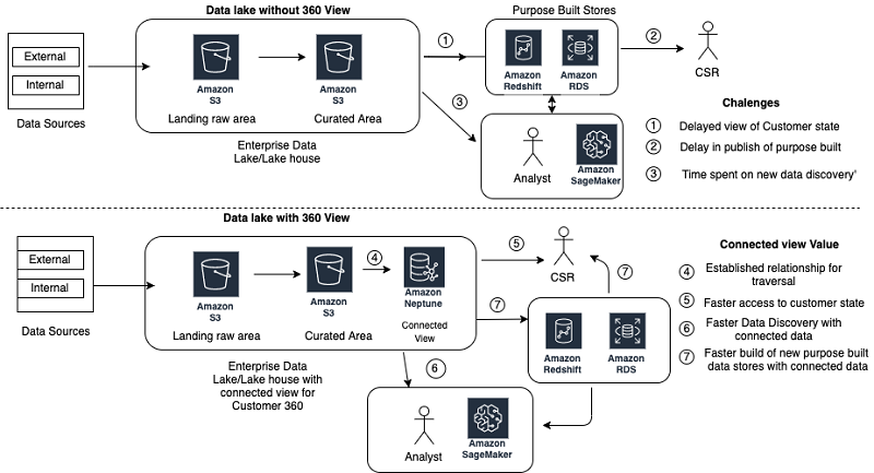
An enterprise data platform ingests customer journey data using a variety of data capture mechanisms (web front ends, mobile applications, call centers, external feeds, external data agencies and partners, cloud fronts, and internal hosted applications). In a typical data platform, to understand customer behavior patterns, you ingest, transform, and curate all variety of data in different types of data stores. You can broadly classify the data source patterns as external structured, external unstructured, internal structured, and internal unstructured. As the data patterns grow and change with new or modified customer-centric products, the customer journey data gets disjointed in multiple data stores. Connecting all the data associated with a customer to provide a holistic data state can be challenging. The insights become stale and the latency to provide the latest customer-focused insights starts growing. Data lakes become swamps, and you need to clean and build new purpose-built stores to address the unresolved business challenges to reduce customer dissatisfaction.

You can capture the relationship between data entities as vertices and associated edges in the curated layer of the enterprise data lake by using the Tinkerpop property graph. With the Neptune capabilities of variable schema (new properties) and extensibility to add new entities (vertex and edge), you can store customer data from new feeds in near real time and publish customer 360 views faster. The following diagram compares these architectures.

Walkthrough

In this post’s use case, your home insurance company wants to understand your customer behavior in a new insurance paradigm that uses modern applications to sign new customers up for home or apartment insurance. You need to understand the current state of a customer’s journey depending on the path taken (web browser, mobile app, or call center) and sell an insurance policy at the right price and coverage, which results in higher satisfaction for a long-lasting, engaged customer.

This post looks at the four different data ingestion patterns, the associated challenges to analyze the unrelated data, how to use Amazon Redshift to analyze and create graph data, and how Neptune can add value to connect the dots between the data to provide a holistic customer 360 view in near real time. The following table summarizes the four ingestion patterns.

Building the sandbox environment

You build a sandbox environment with AWS platform components (Amazon S3, Amazon Redshift, Neptune) to create a POV for a connected data platform. For more information about commands and procedures, see AWS Documentation.

To build your environment, complete the following steps:

1. Create an S3 bucket (cjsandboxpov<last five digits of account>) with the following folders to store example data from the existing data platform:
   • /landingarea – Landing area folder to collect data from all four sources in CSV or Parquet format
   • /neptune_vertex – Neptune load vertex folder to dump CSV load files for dump data regarding graph vertices
   • /neptune_edge – Neptune load edge folder to dump CSV load files for dump data regarding graph edges

   This post uses the S3 bucket name cjsandboxpov99999.

2. Leave all secure bucket policies at their default.
3. Create an Amazon Redshift cluster in your VPC sandbox environment to upload the source data.
   • The cluster size should support data storage twice the size of raw data (for example, select 2 node ds2.xlarge cluster for up to 2 TB of raw data)
   • Associate the IAM role for Amazon Redshift to read and write to the S3 buckets.

   For more information, see Authorizing COPY, UNLOAD, and CREATE EXTERNAL SCHEMA operations using IAM roles.

4. Use the Amazon Redshift query editor to connect to the Amazon Redshift database and create the sandbox schema cjsandbox to define the incoming source objects.
5. Create a Neptune cluster to capture the graph attributes to build a knowledge base:
   • Choose the latest version with a db.r5large cluster with no read replica
   • Choose cjsandbox as the database identifier and select the defaults as options
   • Initiate creation of the Neptune cluster

Discovering the customer journey and capturing key states

The following diagram illustrates the various paths a customer can take on their journey.

In the home insurance landscape for home, apartment, or property insurance, individuals have multiple options to engage with an insurance provider. An individual journey to buy an insurance policy could be simple and fast, using a mobile application for an apartment, or complex based on the size and location of the property with different coverage needs.

Insurance companies support the growing diverse market by providing multiple options (mobile, web, or call center) for initial first contact with potential customers. Your goal is to provide the best customer experience and quickly assist when a customer runs into a challenge or decides to abandon their inquiry.

The best customer experience requires capturing the customer journey state as quickly as possible, so you can provide options for quicker decisions that lead to the customer signing a policy. The goal is to reduce the abandons due to poor user interface experience, complexity of coverage selection, non-availability of optimal choices and cost options, or complexity of navigation in the provided interface. Also, you need to empower your enterprise representatives (sales and service representatives, or application developers) with the latest trends regarding the customer state and metrics to guide the customer to a successful policy purchase.

From the customer journey, you capture the following key states:

• Initial customer information – Email, address, phone
• Call center data – Phone, agent, state
• Web application logs – Session, quote, last state
• Web analytics logs – Visits, page views, page events
• Core journey data – Policy, quote, customer abandon or reject

Capturing the customer journey ER diagram and model graph with vertices and edges

After you define the customer journey states, identify the key transaction entities where the data is captured for the interaction. Build an ER diagram of the known entities and associated relationship with each other. The following diagram illustrates four isolated customer views.

Each data store consists of key fact tables. The following table summarizes the fact tables and their associated key attributes.

After you review the data in the tables and their associated relationships, analyze the ER diagram for key entities for the graph model. Each key table fact acts as the source for the main vertices, such as CUSTOMER, ADDRESS, CALL, QUOTE, SESSION, VISIT, PAGE_VIEW, and PAGE EVENT. Identify other key entities as vertices, which are key attributes to connect different entities, such as PHONE and ZIP. Identify edges between the vertices by referring to the relationship between the tables. The following graph model is based on the identified vertices and edges.

The next key step is to design the graph model to support the Neptune Tinkerpop property graph requirements. Your Neptune database needs a unique ID for each of its vertex and edge entities. You can generate the ID with a combination of the prefix value and current unique business identifier for an entity. The following table describes some examples of the vertex and edge naming standards used to create unique identities for the Neptune database. Vertex entities are associated with three-letter acronyms concatenated with a database unique identifier. The edge name is derived by the direction of edge <from vertex>_<to_vertex_code>_<child unique id> describing one to many relationships between two vertices. Because the primary key values are unique for an entity, concatenating with a prefix makes the value unique across the Neptune database.

Analyzing the curated data for relationships in Amazon Redshift

Amazon Redshift provides a massively parallel processing (MPP) platform to review data patterns in large amounts of data. You can use other programming options like AWS Glue to create Neptune bulk load files for data stored in an Amazon S3-curated data lake. However, Amazon Redshift offers a database platform to analyze the data patterns and find connectivity between disparate sources, and an SQL interface to generate the bulk load files. An SQL interface is preferred for database-centric analysts and avoids the learning curve for building PySpark-based libraries. This post assumes the curated data for the data stores is published in the Amazon S3-based data lake in a CSV or Parquet format. You can load curated data in a data lake into the Amazon Redshift database using the COPY command.

To create a customer table in the sandbox schema, enter the following code:

Create table sandbox.customer (
customer_id number,
email.  varchar(40),
phone  varchar(20),
address_id number,
..);

To copy data from Amazon S3 to the customer table, enter the following code:

copy customer
from 's3://cjsandboxpov9999/landingarea/customer.dat' 
iam_role 'arn:aws:iam::0123456789012:role/MyRedshiftRole';

Dumping vertices and edges dump files to Amazon S3

The Neptune database supports bulk loads using CSV files. Each file needs to have a header record. The vertex file needs to have vertex ID attributes and label attributes as needed. The remaining property attributes need to specify the attribute format for each attribute in the header. The edge dump file needs to have an ID, from vertex ID, to vertex ID, and label as required attributes. The edge data can have additional property attributes.

The following code is a sample session vertex dump record:

~id,session_id:int,marketing_id:String,quote_id:int,date_created:String,~label
SES29557958,29557958,8016200001,16524635,"2019-02-04 21:51:33.229275",session
SES29557961,29557961,pgrcrp,16524645,"2019-02-04 21:51:33.229275",session
SES29557963,29557963,,16524639,"2019-02-04 21:51:33.229275",session
SES29557965,29557965,InternetW,16524638,"2019-02-04 21:51:33.229275",session
SES29557966,29557966,pgrcrp,16524637,"2019-02-04 21:51:33.229275",session
SES29557967,29557967,9003849004,16524642,"2019-02-04 21:51:33.229275",session
SES29557968,29557968,,16524641,"2019-02-04 21:51:33.229275",session
SES29557969,29557969,OLS,16524653,"2019-02-04 21:51:33.229275",session

The following code is a sample session quote edge dump record:

~id,~from,~to,~label
"SESQTE16524635",SES29557958,QTE16524635,has_quote
"SESQTE16524645",SES29557961,QTE16524645,has_quote
"SESQTE16524639",SES29557963,QTE16524639,has_quote
"SESQTE16524638",SES29557965,QTE16524638,has_quote
"SESQTE16524637",SES29557966,QTE16524637,has_quote
"SESQTE16524642",SES29557967,QTE16524642,has_quote

Because all the related data resides in Amazon Redshift, you can use a view definition to simplify the creation of the dump files for Neptune bulk loads. A view definition makes sure the header record is always the first record in the dump file. However, creating dump files to Amazon S3 has some limitations:

• The NULL value in a column makes the entire string null. View uses the NVL function to avoid the challenge of skipping vertices in case one of the attributes has a NULL
• Commas or other unique characters in attribute data invalidate the dump file data format. View uses the replace function to suppress those characters in the data stream.
• The unload command has a limit of 6 GB to create a single dump file. Any overflow files don’t have the header record, which invalidates the Neptune load format. View lets you sort the data by key columns to unload data in chunks, with each chunk having the Neptune format header.

The following example code is a view definition for a vertex source view:

create or replace view sandbox.v_session as
Select * from.                  --- HEADER FORMAT
(select 'header:string,’||.  – sort column to ensure header is first record
~id,‘session_id:int,start_date:string,,quote_id:string,'||.  
‘date_created:string,last_interaction_date:string,policy_effective_date:string,’||
'~label' session_data      --  LABEL attribute
from sandbox.dummy.    – DUMMY table with 1 row
union all
select  'row,’||
‘SES’||id||','||id||’,’||start_date||’,’||quote_id||','||
date_created||’,’||last_interaction_date||’,’||policy_effective_date||’,’||
'session'. – LABEL for vertex
from sandbox.session
 ) 
order by 1, ID;

The following example code is a view definition for an edge source view:

create or replace view sandbox.v_session_quote as
  SELECT * FROM (
    SELECT 'header:string,~id,~from,~to,' || '~label' AS session_quote_data
    FROM sandbox.dummy
    UNION ALL
    SELECT 'row,SESQTE'|| sessionid || ',SES' || sessionid || ',QTE' || quote_id|| ',' ||
    'sess_quote'
    FROM (SELECT c.sessionid, s.quote_id
          FROM sandbox.customer c,
               sandbox.session s,
              sandbox.quote q
              WHERE c.sessionid= s.id AND
                   q.quote_number = s.quote_id )
  ) WHERE 
   ORDER BY 1,2;

To create the vertex and edge dump files, use the UNLOAD command in Amazon Redshift. See the following code:

unload ('select * from sandbox.v_session')
to 's3://cjsandboxpov9999/neptune_vertex/v_session.dat' 
iam_role 'arn:aws:iam::0123456789012:role/MyRedshiftRole'
PARALLEL OFF;

unload ('select * from sandbox.v_session_quote')
to 's3://cjsandboxpov9999/neptune_edge/v_session_quote.dat' 
iam_role 'arn:aws:iam::0123456789012:role/MyRedshiftRole'
NOPARALLEL OFF;

Loading vertices and edges dump files to Neptune database

The vertex and edge dump files are created in two different Amazon S3 folders. The vertex dump files are loaded first as edges, which requires the from and to for an edge to be present in the database. You can load the files one at a time or as a folder. The following code is the Neptune load command:

curl -X POST \
-H 'Content-Type: application/json' \
https://<instance_name>>.us-east-1.neptune.amazonaws.com:8182/loader -d '
{
"source" : "s3://<<<location>> ",
"format" : "csv",
"iamRoleArn" : "ARN for IAM role with access to read from S3 Bucket",
"region" : "us-east-1",
"failOnError" : "FALSE",
"parallelism" : "HIGH"
}’

The load jobs create a distinct loader ID for each job. You can monitor the load job progress by passing the loader ID as a variable to the wget command.

To review the state of the load status, enter the following code:

wget https://<<instance>.us-east-1.neptune.amazonaws.com:8182/loader/{loader_id}?details=true

To review load status with errors, enter the following code:

wget ‘https://<<instance>.us-east-1.neptune.amazonaws.com:8182/loader/{loader_id}?details=true&errors=true’

Performing POV of connected database

You need to verify the new solutions you implemented for their value to address the business outcomes. The connected Neptune database can now create a holistic view for a customer service representative. This post includes an example Python code to describe how to share a customer 360 of the connected data with an end-user. Complete the following steps:

1. Using a customer ID, like email, identify the start vertex. For example, the following code is a Gremlin query:

   g.V().hasLabel(‘customer’). \\ select customer vertex 
   has(email,’xxxx@mail.com’). \\ identify individual through properties 
   valueMap().fold().next())  \\ get all properties

2. Navigate to the address vertex connected to customer vertex and get all associated address information. For example, see the following code:

   g.V().hasLabel('customer').has('email','xxxxxx@mail.com').out().hasLabel('address').project('address','city','zip','state').by('address').by('city').by('zip').by('state').toList()

3. Navigate to all phone vertex and capture all call data in chronological order.
4. Navigate to session and web analytics visit to capture all web activity.
5. Navigate to associated quote and see the pattern for insurance selection.
6. Identify the current state of the customer.

The visualization of a connected universe for a customer’s data provides the greatest value for a Neptune graph database. You can analyze the graph to discover new datasets and data patterns. You can then use these new patterns as input for ML to assist with optimizing the customer journey. The graph database reduces discovery time to understand data patterns for seed data to build ML models.

You can explore the connectivity between different entities by using a graphical browser interface for a graph database. The Show Neighborhood option in most graph browsers allows you to traverse different paths the customer takes. Complete the following steps:

1. Start with a gremlin query to get the customer vertex.
2. To see the associated phone, address, web sessions, and quotes, choose Show neighborhood for the customer vertex.
3. To see all visits for a session, choose Show neighborhood for a session.
4. To see all calls associated with a customer, choose Show neighborhood for a phone.
5. To see all policies associated with a quote, choose Show neighborhood for a quote.
6. To see all associated page views, choose Show neighborhood for a visit.

You can use the connected customer journey view to enhance the user interface (mobile or web) to set default coverage options using most widely selected options for a demographic (one-click insurance). For a zip code or a city, when you traverse the graph, you can identify customers and associated quotes and policies to identify the pattern for the deductibles and coverage chosen by satisfied customers. For abandon analysis, you can select the quotes with no policies to navigate to web analytics and find which form or event triggers customer abandon due to a complex user interface. To reduce call volumes to the call center, traverse the graph to capture trends of events that trigger a customer call.

Integrating the data lake with Neptune

After you establish the value of connected data, you can enhance the daily data pipeline to include the connected Neptune database. After you curate the data and publish it in the data lake, you can glean connected data to add new vertices, edges, and properties. You can trigger AWS Glue jobs to capture new customers, connect new application sessions to customers, and integrate the incremental web analytics data with session and customer information. This post includes an example AWS Glue job for maintaining vertices and edges.

After you publish a new curated data fact, trigger an AWS Lambda function to start an AWS Glue job to capture the latest entities added or modified, make sure their dependent data is already published, and then add or modify the vertex, edge, or property information. For example, when new session data arrives in the curated area of your data lake, initiate a job to add customer session-related entities to the Neptune database.

Code examples

The following code example is for a customer 360 using Python and Gremlin:

#!/usr/bin/python
from __future__  import print_function  # Python 2/3 compatibility
from gremlin_python import statics
from gremlin_python.structure.graph import Graph
from gremlin_python.process.graph_traversal import __
from gremlin_python.process.traversal import *
from gremlin_python.process.strategies import *
from gremlin_python.driver.driver_remote_connection import DriverRemoteConnection
import json
graph = Graph()
### create database connection
remoteConn = DriverRemoteConnection('wss://cjsandbox.xxxxx.us-east-1.neptune.amazonaws.com:8182/gremlin','g')
g = graph.traversal().withRemote(DriverRemoteConnection('wss://cjsandbox.xxxxxx..us-east-1.neptune.amazonaws.com:8182/gremlin','g'))
### run Gremlin queries and store detail in json variables
## get customer data
vcust = g.V().hasLabel('customer').has('email','xxxxxxx@aol.com').project('email','dob').by('email').by('dob').toList()
## get session data
vcount = g.V().hasLabel('customer').has('email','xxxxxxx@aol.com').out().hasLabel('session').count().toList()
vqcount = g.V().hasLabel('customer').has('email','xxxxxxx@aol.com').out().hasLabel('quote').count().toList()
## get address count and  data
vaddcount = g.V().hasLabel('customer').has('email','xxxxxxxx@aol.com').out().hasLabel('address').count().toList()
vaddress = g.V().hasLabel('customer').has('email','xxxxxx@aol.com').out().hasLabel('address').project('address','city','zip','state').by('address').by('city').by('zip').by('state').toList()
v_fullcust=format(g.V().hasLabel('customer').has('email','xxxxx@aol.com').valueMap().fold().next())
vsess= g.V().hasLabel('customer').has('email','XXXX@aol.com').out().hasLabel('session').order().by('start_date').project('start_date','session_id','partner_id').by('start_date').by('session_id').by('partner_id').toList()
vcust_json = json.dumps(vcust[0])
vcount_json = json.dumps(vcount[0])
vaddcount_json = json.dumps(vaddcount[0])
vsesscount = json.loads(vcount_json)
vaddrcount = json.loads(vaddcount_json)
### print customer information
print("====== Customer Information=========================")
print("====== Customer Information=========================")
print(" Email:  %s " % json.loads(vcust_json)['email'])
print(" Date of birth: %s " % json.loads(vcust_json)['dob'])
print(" Number of sessions:   %s sessions  " % vsesscount)
print(" Number of properties:   %s   " % vaddcount)
print(" Property Address details: :    " )
for i in range(vaddrcount,0,-1):
        address_json= json.dumps(vaddress[i-1])
        print(address_json)
print(" Customer misc details :  ")
print(v_fullcust)
print("-----------------------------------------------------\n\n")
print("====== Custoner session Information =====sorted by date creation descending ========== " )
### print session by looping
for i in range(vsesscount,0,-1):
        vsess_json= json.dumps(vsess[i-1])
        print("Session : ")
        vsessid=json.loads(vsess_json)['session_id']
        print(vsess_json)
        vsessinfo=g.V().has('session','session_id',vsessid).valueMap().select('date_created','policy_effective_date','marketing_id','form_number').fold().next()
        print(vsessinfo)
        print("--------------------------\n ")
remoteConn.close()

The following code example is an AWS Glue program that creates a Neptune CSV file as incremental data is curated:

import sys
import boto3
import logging
###awsglue libs
from awsglue.utils import getResolvedOptions
from awsglue.transforms import ApplyMapping
from awsglue.transforms import RenameField
from awsglue.transforms import SelectFields
from awsglue.dynamicframe import DynamicFrame
from awsglue.context import GlueContext
from awsglue.job import Job
##pyspark libs
from pyspark.context import SparkContext
from pyspark.sql.functions import lit
from pyspark.sql.functions import format_string
## add lib
sc = SparkContext()
#sc.addPyFile("s3://aws-glue-scripts-999999-us-east-1/glue_neptune/glue_neptune.zip")
### gremlin/glue_neptune needs zip library
from gremlin_python import statics
from gremlin_python.structure.graph import Graph
from gremlin_python.process.graph_traversal import __
from gremlin_python.process.strategies import *
from gremlin_python.driver.driver_remote_connection import DriverRemoteConnection
from gremlin_python.process.traversal import *
from glue_neptune.NeptuneConnectionInfo import NeptuneConnectionInfo
from glue_neptune.NeptuneGremlinClient import NeptuneGremlinClient
from glue_neptune.GremlinCsvTransforms import GremlinCsvTransforms
####
###Logging Context
MSG_FORMAT = '%(asctime)s %(levelname)s %(name)s: %(message)s'
DATETIME_FORMAT = '%Y-%m-%d %H:%M:%S'
logging.basicConfig(format=MSG_FORMAT, datefmt=DATETIME_FORMAT)
logger = logging.getLogger("cjsandboxglue")
logger.setLevel(logging.INFO)
logger.info("Hello from glue message")
####
args = getResolvedOptions(sys.argv, ['JOB_NAME', 'S3_OUTPUT_PATH','DATABASE_NAME','TABLE_NAME','PIPELINE_ID','PIPELINE_JOB_ID"])
glueContext = GlueContext(sc)
job = Job(glueContext)
job.init(args['JOB_NAME'], args)
nodes_path = '{}nodes'.format(args['S3_OUTPUT_PATH'])
edges_path = '{}edges'.format(args['S3_OUTPUT_PATH'])
jobname= args['JOB_NAME']
database = args['DATABASE_NAME']
session_table = args['TABLE_NAME']
pipelinename = args['PIPELINE_ID']
jpbid = args['PIPLEINE_JOB_ID']
def writeCsvFile(datasource, path):
    dataframe = DynamicFrame.toDF(datasource).repartition(1)
    datasource = DynamicFrame.fromDF(dataframe, glueContext, 'write-csv')
    glueContext.write_dynamic_frame.from_options(frame = datasource, connection_type = "s3", connection_options = {"path": path}, format = "csv", transformation_ctx = "write-csv")
# Arguments
print ("job name =", jobname)
print ("s3 path =",nodes_path)
print ("table prefix= ",session_table)
print ("catalog database= ",database)
print ("pipeline= ",pipelinename)
print ("job id = ",jobid)
datasource0 = glueContext.create_dynamic_frame.from_catalog(database = database, table_name = session_table, transformation_ctx = "datasource0")
applymapping1 = ApplyMapping.apply(frame = datasource0, mappings = [("session_id", "bigint", "session_id:int", "int"), ("marketing_id", "string", "marketing_id:String", "string"), ("quote_id", "bigint", "quote_id:int", "int"), ("date_created", "string", "date_created:String", "string")], transformation_ctx = "applymapping1")
applymapping1 = GremlinCsvTransforms.create_prefixed_columns(applymapping1, [('~id', 'session_id:int', 'SES'),('~to', 'quote_id:int', 'QTE')])
selectfields1 = SelectFields.apply(frame = applymapping1, paths = ["~id", "session_id:int", "marketing_id:String", "quote_id:int", "date_created:String"], transformation_ctx = "selectfields1")
writeCsvFile(GremlinCsvTransforms.addLabel(selectfields1, 'session'), nodes_path)
# Edges
applymapping1 = RenameField.apply(applymapping1, "~id", "~from")
applymapping1 = GremlinCsvTransforms.create_edge_id_column(applymapping1, '~from', '~to')
selectfields2 = SelectFields.apply(frame = applymapping1, paths = ["~id", "~from", "~to"], transformation_ctx = "selectfields2")
writeCsvFile(GremlinCsvTransforms.addLabel(selectfields2, 'has_quote'), edges_path)
# End
job.commit()

Conclusion

You can use Neptune to build an enterprise knowledge base for a customer 360 solution that connects disparate data sources for customer state dashboards, enhanced analytics, online recommendation engines, and cohort trend analysis.

A customer 360 solution with a Neptune database provides the following benefits:

• Access to all activities in near-real time performed by a customer during their journey. You can traverse the graph to better support the customer
• Ability to build a recommendation engine to assist customers during their journey with feedback based on preferences of similar cohorts based on demographics, location, and preferences
• Segmentation analysis based on geography and demographics to understand challenges with the current market and opportunities for new markets
• Business case analysis to narrow down on a challenge by traversing the neighborhood to triage factors affecting your business
• Testing and validating new application deployment effectiveness to improve the customer journey experience

You can apply this solution to similar knowledge bases, such as vehicles or accounts. For example, a vehicle 360 knowledge base can track a journey of an automobile customer from pre-sales, dealer interactions, regular maintenance, warranty, recalls, and resell to calculate the best incentive value for a vehicle.

About the Author

Ram Bhandarkar is a Sr Data Architect with AWS Professional Services. Ram specializes in designing and deploying large-scale AWS data platforms (Data Lake, NoSQL, Amazon Redshift). He also assists in migrating large-scale legacy Oracle databases and DW platforms to AWS Cloud.