AWS Database Blog
Running pgvector in production on Amazon Aurora PostgreSQL
Running pgvector on Amazon Aurora PostgreSQL-Compatible Edition gives you a production-grade vector store on a database you already know, backed by the operational tooling, high availability, and scaling behaviour of Amazon Aurora. That combination is why pgvector has become a common choice for Retrieval Augmented Generation (RAG) workloads moving from proof of concept into production with Service Level Agreements (SLAs). Production traffic does introduce a predictable set of operational considerations: query latency as the corpus grows, recall on filtered vector searches, memory headroom during index builds, and connection behaviour under load. This post is scoped to the database operations that keep the RAG retrieval layer healthy. Model customization through fine-tuning or continued pre-training is out of scope.
In this post, we cover the operational practices that keep a pgvector workload healthy once you depend on it: choosing the right index and distance function, scaling with quantization and partitioning, managing Hierarchical Navigable Small World (HNSW) churn, sizing for memory-resident operation, and the observability signals that catch problems early.
How this post is organized
First, choose an index type (HNSW or Inverted File with Flat Compression) for your dataset and write pattern. Second, set up a baseline schema and query with the AWS-recommended parameters. Third, pick a distance operator that matches your embedding model. Fourth, scale the index to your target dataset size with quantization, parameter tuning, and partitioning. Fifth, plan for churn, capacity, and observability before traffic arrives. Each section builds on the one before.
The examples throughout use a multi-tenant document-store schema on Aurora PostgreSQL-Compatible with Amazon Titan Text Embeddings V2, an Amazon Bedrock foundation model, as the embedding model. Each SQL example is runnable against an Aurora PostgreSQL-Compatible cluster with the vector extension enabled.
This post covers the self-managed path, where you are responsible for the vector store and retrieval pipeline. For a fully managed RAG capability that handles ingestion, embedding, and retrieval for you, use Amazon Bedrock Knowledge Bases, which supports Amazon Aurora PostgreSQL with pgvector as one of its vector store options.
Prerequisites
To follow the examples in this post, you need:
- An Aurora PostgreSQL-Compatible cluster running PostgreSQL version 17.4+, 16.8+, 15.12+, 14.17+, or 13.20+, which supports pgvector 0.8.0. pgvector 0.8.0 is available in all AWS commercial Regions and AWS GovCloud (US) Regions, except AWS China Regions. For the launch details, see the pgvector 0.8.0 Aurora announcement. For the current Region list, see the Aurora PostgreSQL extension versions page.
- The vector extension enabled on your database.
- An embedding model. The examples assume Amazon Titan Text Embeddings V2, a foundation model available through Amazon Bedrock that produces 1024-dimensional embeddings by default.
Choosing the right index strategy
pgvector ships two Approximate Nearest Neighbor (ANN) index types: HNSW and IVFFlat. Both trade perfect accuracy for speed, because a brute-force exact search across millions of vectors is too slow for online queries. The AWS Prescriptive Guidance on vector database options covers where pgvector fits among AWS vector stores. The Self-managed multi-tenant vector search with Amazon Aurora PostgreSQL post walks through the pgvector basics if you want a refresher on the terminology.
For production RAG on Aurora PostgreSQL, HNSW is the default choice for most workloads. But there are two cases where the right answer is no index at all: small datasets, and partitioned datasets where 100% recall is required. The rest of this section explains why HNSW wins for the common case, when IVFFlat still makes sense, and when skipping the index entirely is the correct production decision.
How HNSW works, and why it is the default
HNSW stands for Hierarchical Navigable Small World. It builds a multi-layer proximity graph. Layer 0 contains every vector, densely connected to its nearest neighbors. Each higher layer samples a smaller subset of vectors with longer-range connections. A single vector is the entry point, present in every layer. For a detailed walk-through of both HNSW and IVFFlat internals beyond the summary here, see the deep dive into IVFFlat and HNSW techniques.
A search starts at the entry point in the top layer. Within a layer, pgvector performs a greedy best-first walk along the graph edges, moving to whichever connected neighbor is closest to the query vector. When it can no longer get closer, it descends to the same node in the layer below and continues the walk there. At layer 0 the walk expands into a beam search controlled by the hnsw.ef_search parameter, and the top candidates are returned.
The following diagram shows that descent in action, from the entry point at the top layer down to the beam search at layer 0.
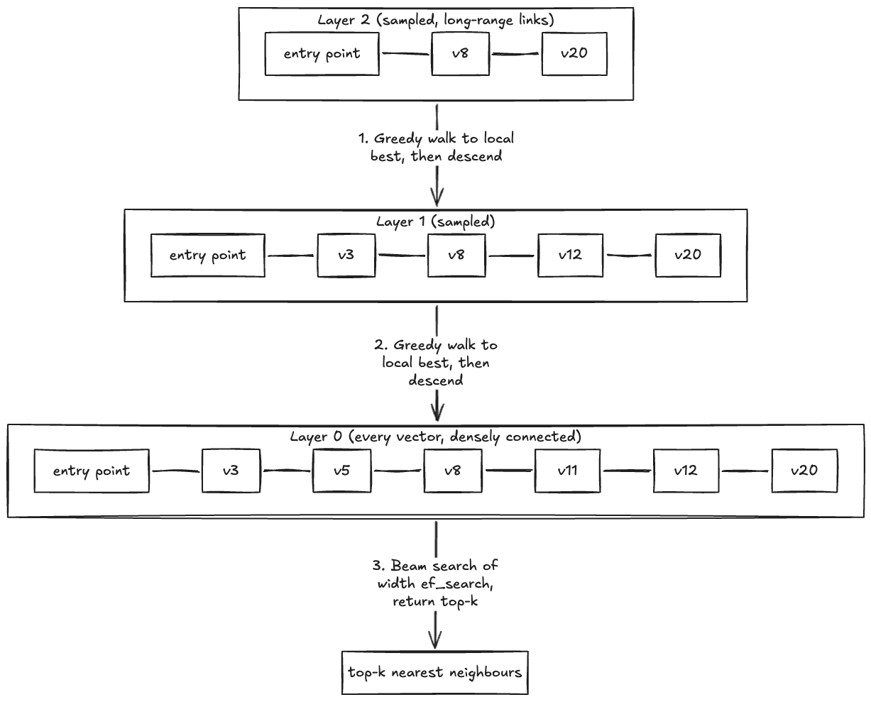
HNSW layered descent. A query enters at the entry point in the top layer, performs a greedy walk within each layer to find the local nearest neighbor, descends to the same node in the layer below, and expands into a beam search at layer 0 to return the top-k results.
This structure makes HNSW fast to query and lets it accept inserts incrementally. You can write new vectors directly into a live index without pausing or batching. Recall and latency are controlled at query time through hnsw.ef_search, so you can tune per workload without rebuilding the index.
The trade-off is build cost. HNSW indexes take longer to build and use more memory than IVFFlat, because the graph itself must be stored alongside the vectors. For the production RAG pattern this post targets, the trade-off is worth it: you build the index once, and queries stay fast provided you manage churn (covered later in the Managing index churn section).
When IVFFlat still makes sense
IVFFlat stands for Inverted File with Flat compression. Instead of a graph, it groups vectors into clusters using k-means. Each cluster has a representative point at its center, called a centroid. At query time, pgvector compares the query vector to the centroids, picks the nearest clusters, and searches only inside those clusters.
The following diagram shows the space partitioned into clusters, with a query compared against the centroids and then against the vectors inside the nearest clusters.
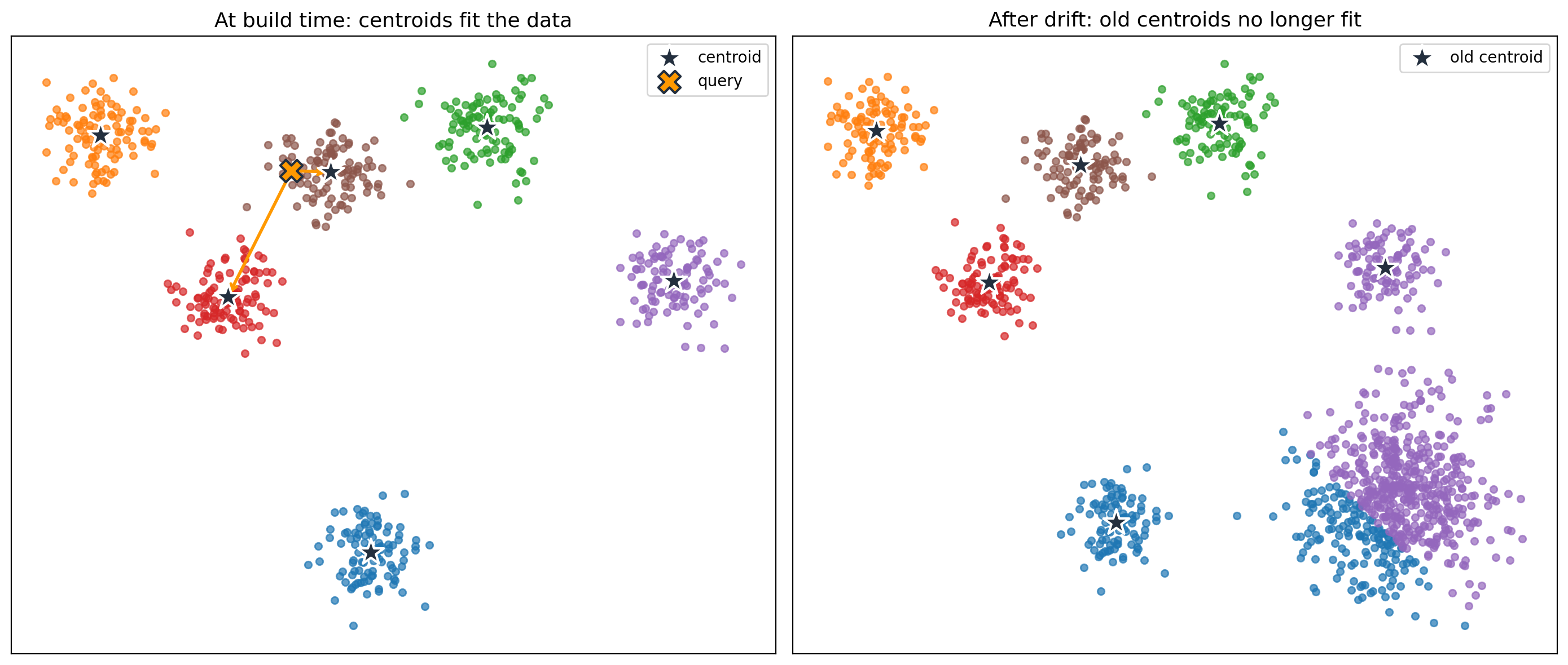
IVFFlat is cheaper to build than HNSW: clustering is simpler than graph construction, and the index stores no graph, so it uses less memory. However, IVFFlat fixes the centroids at build time. If your data changes after the index is built, new vectors might not match the existing clusters well, and recall drops. The fix is to rebuild the index, which recomputes the centroids against the current data. Centroid retraining means re-running k-means over the full dataset to produce a fresh set of cluster centers.
IVFFlat fits a narrow set of workloads: large, mostly static corpora with an existing batch rebuild schedule. Everything else belongs on HNSW.
When no index is the right choice
There are two production patterns where no index outperforms either ANN option.
The first is the small-dataset case. For tables with roughly 10,000 to 50,000 vectors, a parallel sequential scan is fast enough on its own, and skipping the index avoids build time, maintenance cost, and the recall loss inherent to approximate search. This is the case called out in the pgvector 0.8.0 best practices, and it is the usual starting point for new workloads before the corpus grows.
The second is the partitioned, recall-critical case. If your schema partitions data so that every query touches a bounded subset (for example, per tenant or per user), and your use case requires 100% recall, a brute-force parallel scan within a partition can beat an ANN index. The Ring engineering team runs exactly this pattern in production: 100 to 200 billion embeddings are spread across per-user partitions of roughly 1 GB each. Each partition is scanned with max_parallel_workers_per_gather = 16, with no vector index at all. Removing the index was the change that let PostgreSQL pick parallel sequential scans over single-threaded index scans, which drove EBS throughput from about 50 MB/s to nearly 500 MB/s. Full details are in the Ring billion-scale semantic video search post.
Two conditions must hold for this pattern to work. First, the per-partition scan has to fit the latency budget, which in practice means each partition stays small enough to be served mostly from the buffer cache or local NVMe. Second, your workload must genuinely need 100% recall. If the ANN recall achievable with HNSW is acceptable, HNSW is simpler and faster. When both conditions are met, skipping the index removes an entire class of operational concerns: no build cost, no churn management, no memory sizing for index pages.
Quick decision guide
The following flowchart summarises the decision, starting from dataset size and walking through write pattern, HNSW build cost, and partitioning to a concrete index choice.
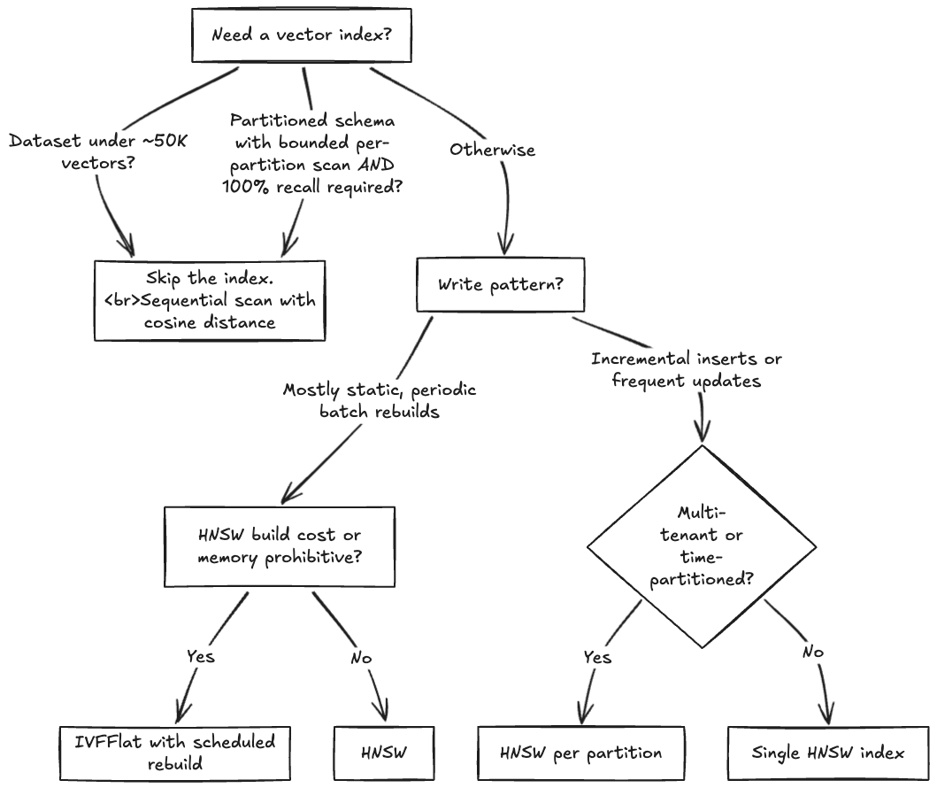
The “skip the index” branch covers both cases from the previous section: small tables where a sequential scan is already fast enough, and partitioned schemas where 100% recall is required within a bounded per-partition scan. Ring runs the second pattern in production, with per-customer partitions so every search reads only that customer’s data. For how they designed for it, see the preceding no-index discussion and the Ring billion-scale semantic video search post.
A runnable baseline
Before going deeper into similarity functions and scaling, here is a baseline schema, index, and query that the rest of the post builds on. It reflects the AWS-recommended HNSW parameters from the pgvector 0.8.0 best practices section and the iterative scan default we recommend for production.
The baseline uses HNSW, which fits the common production RAG case: per-tenant partitions are large enough that a sequential scan is not competitive, and ANN recall at the default settings is acceptable. If your workload looks like the no-index pattern covered earlier, small tables, or partitioned schemas where 100% recall is required within a bounded per-partition scan, omit the HNSW index from the following example and keep the rest of the schema as shown.
On a populated documents table, this returns up to 10 rows ordered by cosine distance:
| id | content |
| 42 | Q3 revenue grew 18% year over year, driven by enterprise… |
| 117 | The FY26 capital plan was approved at the November board… |
| 203 | Customer churn declined to 2.1% following the support model… |
| … | … |
| (10 rows) | |
In production code, wrap the two SET statements and the SELECT in a transaction and use SET LOCAL instead, so the values apply only to that query rather than the whole session. Swap vector_cosine_ops for vector_ip_ops (and the <=> operator for <#>) if your embeddings are unit-normalized. The next section explains when each choice applies.
Similarity functions at scale
pgvector supports several distance operators. The three that matter for text and semantic embeddings are listed in the following table. Each operator is paired with a specific HNSW operator class at index-creation time. If you use the wrong pair, the planner cannot use the index.
| Operator | Meaning | HNSW operator class | When to use |
| <=> | Cosine distance | vector_cosine_ops |
Safe default for text or semantic embeddings. Ignores vector magnitude. |
| <#> | Negative inner product | vector_ip_ops |
Faster than cosine when vectors are already unit-normalized. |
| <-> | L2 (Euclidean) distance | vector_l2_ops |
Rarely appropriate for semantic search. |
A note on <#>: pgvector returns the negative inner product because PostgreSQL can only use ASC-order index scans. This means ORDER BY embedding <#> query ASC returns the most similar vectors first. If you want a positive similarity score in the result, multiply by -1: SELECT (embedding <#> query) * -1 AS similarity.
Picking cosine or inner product
Amazon Titan Text Embeddings V2 normalizes by default through the normalize API parameter, which defaults to true. For Amazon Titan Text Embeddings V2 output with the default settings, inner product (<#>) is the right choice. On normalized vectors, cosine and inner product produce identical rankings, because cosine divides the inner product by the product of the vector norms, and for unit vectors that divisor is always 1. The norms and division still get computed per comparison, but inner product skips that work. If you override normalize to false, or use an embedding model that does not normalize (such as BGE or older Sentence-Transformers models), fall back to cosine.
Verify that your stored vectors are actually unit-normalized before switching operators. Norm should be 1.0 within floating-point tolerance:
If one or more rows return a norm that is materially different from 1.0, your data is not normalized and the <#> shortcut will produce wrong results. The greatest(0, …) guard protects against sqrt of a tiny negative floating-point residual for vectors that are unit-normalized within tolerance.
Iterative scans for filtered queries
pgvector 0.8.0 introduced iterative index scans, which fix the overfiltering problem. Before 0.8.0, a query that combined a WHERE clause with a vector search often returned fewer results than the LIMIT asked for, because the index returned its top-k candidates before the filter was applied and most candidates were filtered out.
Iterative scans keep pulling candidates from the index until the query satisfies the filter or hits a configurable limit. Three modes are available:
- off: the pre-0.8.0 behavior. Fastest, but can under-return.
- strict_order: preserves exact distance ordering. Safer, but slower for selective filters.
- relaxed_order: returns the correct count with approximate ordering within the result set. We recommend this mode for most production use cases.
Two related parameters bound the scan when you enable iterative mode: hnsw.max_scan_tuples (default 20,000) caps how far the scan walks the index, and hnsw.scan_mem_multiplier (default 1) caps how much memory the scan uses as a multiple of work_mem. Raise scan_mem_multiplier first if max_scan_tuples increases alone do not improve recall for a filtered query.
Scaling to millions of vectors
Three levers matter when the dataset grows beyond a few hundred thousand vectors: quantization, HNSW parameter tuning, and partitioning.
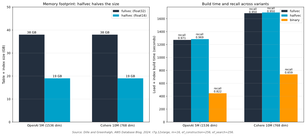
Quantization reduces memory footprint at a small cost to recall. pgvector supports halfvec (16-bit floats) and binary quantization. The AWS pgvector 0.7.0 benchmarks show halfvec cuts memory roughly in half with minimal recall loss, and binary quantization produces large build speed-ups at the cost of recall that you recover with a re-ranking pass, shown in the next subsection. For most workloads, start with halfvec. Move to binary quantization only when you already have a re-rank pipeline in place.
The benchmarks used OpenAI (5M vectors, 1536 dimensions) and Cohere (10M vectors, 768 dimensions) datasets. Amazon Titan Text Embeddings V2 at 1024 dimensions sits between them, so the memory and build-time trade-offs should apply proportionally. Validate against your own data before committing to a quantization strategy.
The following chart shows the memory and recall trade-off across float32, halfvec, and binary representations on those benchmarks.
Two-stage retrieval with binary quantization
An HNSW index and its full-precision vectors must stay memory-resident for performance. When the working set exceeds what RAM can hold, the choices are to shrink the in-memory representation (quantization), extend effective memory with Aurora Optimized Reads, or both. Binary quantization with re-ranking does the shrinking: coarse candidate selection runs on tiny binary vectors that fit easily, and re-ranking by cosine distance pulls full-precision vectors only for the final top-N.
The following SQL pattern implements that two-stage retrieval: Hamming distance for the coarse pass, cosine distance for the re-rank. The re-rank is what recovers most of the recall lost to quantization.
The outer query sees only the 100 coarse candidates, so the expensive cosine comparison runs on a small set. The inline binary_quantize() cast is shown for clarity. For production at scale, materialize the binary vectors in a stored column and index them with bit_hamming_ops so the coarse pass uses an index rather than computing the quantization at query time. For benchmarks of this pattern on pgvector 0.8.0 and Aurora, see Supercharging vector search performance and relevance with pgvector 0.8.0 on Amazon Aurora PostgreSQL.
HNSW exposes three parameters worth tuning:
m: max connections per layer. Higher values improve recall but increase memory use and build time. AWS recommendsm = 16as the starting point.ef_construction: dynamic candidate list size during build. Higher values improve index quality at build time. AWS recommendsef_construction = 128. The pgvector default is 64.ef_search: dynamic candidate list size during query. Higher values improve recall at query latency cost. The pgvector default is 40, which is often too low for production. Tune per workload. Do not hardcode.
Partitioning keeps individual indexes manageable. Partition by tenant for multi-tenant workloads, by time for append-heavy workloads such as event or log data, or by category when queries are scoped to a known subset. Partitioning also supports parallel index builds and per-partition rebuilds.
For bulk loads, defer indexing. Load the data first, then build the index once at the end. Inserting into a live HNSW index is slower than a single post-load build, and the resulting index is often better structured.
When the working set outgrows RAM
RAM residency is the first target, but at some dataset sizes keeping the entire HNSW graph in shared_buffers stops being economical. Aurora Optimized Reads extends effective cache capacity by up to 5x the instance memory using local NVMe storage as a tiered cache, with up to 8x lower read latency for queries that would otherwise fetch from Aurora storage. The feature documentation lists pgvector nearest-neighbor search across millions of vector embeddings as a target use case.
Optimized Reads tiered cache requires an Aurora I/O-Optimized cluster on an NVMe-backed instance family (r6gd, r8gd, or r6id) and is enabled automatically on those instance classes. On an Aurora Standard cluster, Optimized Reads provides only temporary object acceleration, not tiered cache. Monitor the AuroraOptimizedReadsCacheHitRatio Amazon CloudWatch metric alongside BufferCacheHitRatio to see how much of the traffic misses RAM but still hits NVMe rather than storage.
Treat tiered cache as an extension of the memory budget, not a substitute for it: RAM is still faster than NVMe, and NVMe is still faster than Aurora storage. Size the instance so the hot working set stays in RAM, and let Optimized Reads absorb the long tail.
Managing index churn
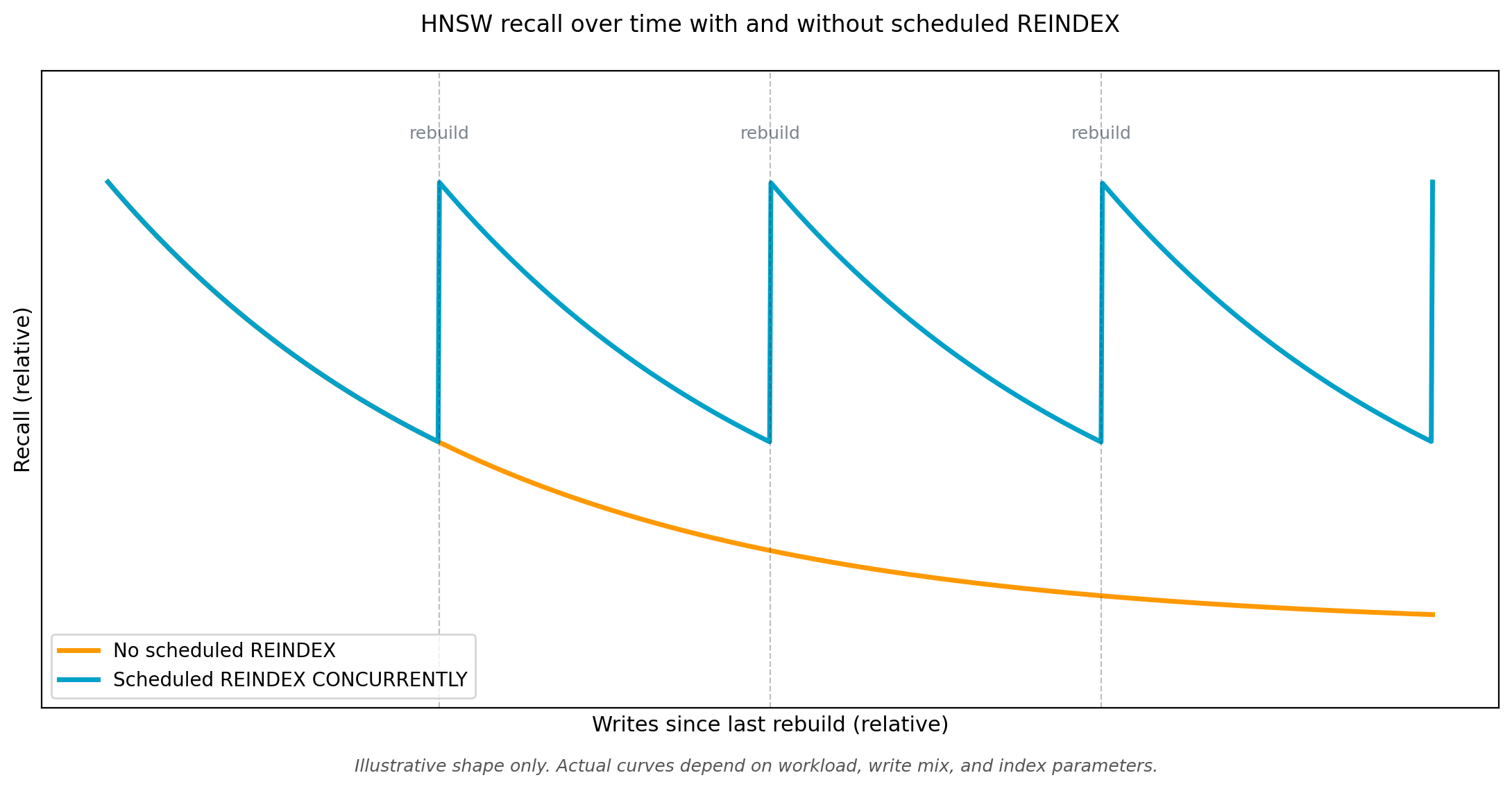
HNSW indexes degrade with deletes and updates. Each change leaves an invalid entry in the graph. Over time, this hurts recall and inflates index size. There is no in-place compaction.
The following chart illustrates how recall drifts downward between rebuilds and recovers at each scheduled REINDEX CONCURRENTLY.
Three patterns work in production:
REINDEX CONCURRENTLY rebuilds the index without blocking writes, but is resource-intensive. Schedule it during low-traffic windows and monitor maintenance_work_mem headroom. For large indexes, plan hours, not minutes.
Partition-based rebuilds are often cleaner. If you partition by time, you can drop and rebuild an entire partition’s index in one operation rather than churning a monolithic graph. This also caps the scope of a failed rebuild.
Append-only with periodic compaction suits workloads where old data becomes irrelevant. Write new vectors to an active partition, then periodically move or drop older partitions. The active index stays small and fast.
Your write pattern determines which one to pick. Workloads that are mostly inserts with few updates do fine on a scheduled REINDEX CONCURRENTLY. Workloads with heavy updates or deletes are better served by partitioning (by time or by batch) and rebuilding partitions independently. Workloads where relevance is time-bounded, for example a search over only the last 90 days, suit the append-only pattern with periodic compaction of old partitions.
Capacity planning
Churn management determines how often the graph is rebuilt. Capacity planning determines whether each rebuild and each query has the memory it needs. The two go together.
An HNSW index must stay memory-resident. When it spills to disk, search latency degrades, because the graph traversal pattern is random and each miss is a page fault. Plan for the index to fit in RAM with headroom for concurrent queries and maintenance operations.
The HNSW graph consumes more memory than the raw vector data, driven primarily by the m parameter. Size Aurora instances to keep shared_buffers plus connection and work memory below the instance’s available RAM.
Choose a memory-optimized instance class for Aurora PostgreSQL vector workloads, since the HNSW graph must fit in RAM. The Amazon Relational Database Service (Amazon RDS) r-series instance families are sized for memory-bound workloads such as vector search. For the current list of supported instance classes, see the Aurora DB instance classes documentation.
Tune these PostgreSQL parameters:
shared_buffers: Aurora sets a reasonable default, but verify it covers your expected index working set.effective_cache_size: signals the query planner about available OS-level cache. Set to roughly 75% of instance memory on Aurora.maintenance_work_mem: critical during index builds. Too low, andCREATE INDEXor REINDEX spill and slow down. pgvector emits aNOTICEwhen the HNSW graph no longer fits inmaintenance_work_mem. If you see it in your build logs, raise the parameter on the instance and re-run the build.work_mem: per-operation. With many concurrent vector queries, lowwork_memcauses spills. Too high a value risks memory pressure under load.max_parallel_maintenance_workers: pgvector 0.7.0 added parallel HNSW builds. Set this to take advantage of larger instances during index creation.
For pricing, see the Amazon Aurora pricing page.
Observability
You cannot tune what you cannot see. Four observability layers matter for pgvector: query-level statistics, instance-level metrics, wait-event analysis, and application-defined custom metrics. Connection handling rounds them out.
Query-level statistics come from pg_stat_statements and the Aurora-specific aurora_stat_statements function. The Aurora variant adds storage I/O and peak memory columns, which matter for vector queries because a spilling search looks different in I/O than a cached one. To find the top vector queries by total time and peak memory:
total_exec_time is in milliseconds and max_exec_peakmem is in bytes. The peak memory columns require Aurora PostgreSQL 16.3, 15.7, or 14.12 and higher. On earlier minor versions, remove max_exec_peakmem from the SELECT list.
Instance-level metrics in CloudWatch tell you whether the index fits in memory. Watch BufferCacheHitRatio (should stay above 99% for healthy vector workloads), SwapUsage (should be zero), and ReadIOPS (sustained high values on a read-heavy vector workload suggest the index is spilling).
Amazon CloudWatch Database Insights surfaces slow queries with wait event breakdowns. Use it to find vector queries blocked on I/O or lock contention.
Custom metrics close the gap between database health and application health. Two are worth building:
- Recall tracking: periodically run a fixed set of evaluation queries whose correct top-k results you know, compare what pgvector returns against the known correct set, and emit the recall percentage to CloudWatch. Drops in recall indicate index drift or query parameter regression.
- p99 latency for vector searches, tagged by query type. Tail latency on vector search often moves before CPU or memory metrics do, because a handful of queries that evict the HNSW graph from cache can degrade recall and latency without changing averages.
Connection handling also needs monitoring. Vector queries are memory-heavy, so an over-subscribed connection pool exhausts work_mem quickly. Use Amazon RDS Proxy in front of Aurora and watch DatabaseConnections, ClientConnections, and MaxDatabaseConnectionsAllowed.
Clean up
If you created the baseline documents table and its indexes to follow along with the examples, remove them when you are done to avoid incurring ongoing storage charges for unused data:
The vector extension does not incur charges on its own, but if you enabled it only for these examples, you can remove it with DROP EXTENSION IF EXISTS vector;. Do not drop the extension if other databases in the cluster are using it.
If you provisioned a dedicated Aurora PostgreSQL-Compatible cluster for testing, delete the cluster and its automated backups with the AWS Command Line Interface (AWS CLI) once you are done. Aurora PostgreSQL-Compatible clusters incur charges for as long as they exist, including storage charges on stopped clusters, so delete the cluster after testing to stop these charges:
Manual snapshots persist after a cluster is deleted and continue to incur storage charges until you delete them explicitly. If you took any during testing, remove them:
Replace , , and with the values from your test environment. The --skip-final-snapshot flag is appropriate for a disposable test cluster. Do not use it on a cluster that holds data you want to keep.
Key takeaways
Before going live, verify these five:
- Plan for HNSW rebuilds from day one. Choose
REINDEX CONCURRENTLYon a schedule, partition-based rebuilds, or append-only with compaction based on your write pattern. - Set
hnsw.ef_searchexplicitly at session or query level. The default (40) is often too low for production recall. A value of 100 is a sensible starting point. - Size
maintenance_work_memto cover your largest index build, with headroom. A build that spills to disk produces a lower-quality graph. - Account for concurrent vector searches when sizing connection quotas. Each concurrent query consumes
work_mem. Multiply out and use Amazon RDS Proxy in front of the cluster. - Treat
BufferCacheHitRatioas the first metric to check. It is the earliest signal that an index has outgrown its instance.
Conclusion
Running pgvector on Amazon Aurora PostgreSQL at production scale rewards teams who design for their workload up front. Corpus size, write mix, filter patterns, and recall targets shape the right index choice, parameter settings, and capacity plan. The sooner you make those decisions deliberately, the smoother the path from proof of concept to SLA-backed production.
In this post, we covered the operational practices that matter: picking the right index and distance function, scaling with quantization and partitioning, managing HNSW churn, sizing for memory-resident operation, and the observability signals that catch problems early. Treat this as a checklist for your first production rollout, and revisit it when traffic or dataset size doubles.