Scale pgvector with binary quantization on Amazon Aurora PostgreSQL

Customers building AI-powered applications on Amazon Aurora PostgreSQL-Compatible and Amazon Relational Database Service (Amazon RDS) for PostgreSQL with pgvector are scaling vector workloads into the hundreds of millions and billions. Ring, for example, stores between 100-200 billion embeddings and ingests approximately 2 billion new embeddings daily for semantic video search on Amazon RDS for PostgreSQL (read the Ring blog post). When your HNSW index grows past available instance memory, most queries incur disk I/O at the lower graph layers and latency degrades from milliseconds to seconds. Binary quantization with reranking offers a practical tradeoff: it compresses each vector to a single bit per dimension, shrinking a 100-million-vector index from 367 GB to ~38 GB so it can fit in the buffer cache of standard instances. A reranking step rescores the top candidates against full-precision vectors to partially recover the accuracy lost during compression. Some recall loss is inherent, because relevant results excluded in the initial binary search cannot be recovered. In this post, we show you how to implement binary quantization with reranking on Amazon Aurora PostgreSQL using the built-in support in pgvector. We provide practical guidance on sizing, validation, and the scenarios where this approach works best.

This guidance is based on three indexing approaches evaluated across public datasets at scales from 5 million to 100 million vectors on memory-constrained instances. The recommendation: HNSW with binary quantization is the most effective path for customers whose datasets exceed available instance memory. It delivers comparable or better performance than alternative disk-based approaches with significantly faster index builds and no additional extension dependencies.

Prerequisites

To follow along with this post, you need:

• An Amazon Aurora PostgreSQL cluster running Aurora PostgreSQL 16.8 or later (which ships pgvector 0.8.0+), or Aurora PostgreSQL 17.x. pgvector 0.8.0 introduces iterative index scans (hnsw.iterative_scan), required for reranking depths beyond 1,000 candidates as shown in this post.
• An Aurora I/O-Optimized cluster configuration. The NVMe tiered-cache capabilities discussed in the sizing section (Aurora Optimized Reads) require I/O-Optimized. Standard clusters use NVMe only for temporary objects.
• Familiarity with pgvector index types (HNSW, IVFFlat) and basic vector search concepts (recall, approximate nearest neighbor)
• An Aurora instance with sufficient memory for your dataset (see the sizing guidance section for recommendations)
• A vector dataset loaded into a table with a vector column. The examples in this post use 768-dimension and 1536-dimension embeddings, but the approach works at other dimensions supported by pgvector.

How binary quantization with reranking works

HNSW is pgvector’s graph-based index and the most common choice for approximate nearest neighbor search. It builds an in-memory graph that delivers the highest recall and lowest latency when the index fits entirely in the PostgreSQL buffer cache. The tradeoff: a 100-million-vector index at 768 dimensions consumes approximately 367 GB, which requires you to scale up to larger, more expensive instance types (such as r8g.16xlarge with 512 GB RAM) rather than running on the more affordable instance sizes most workloads use.

HNSW with binary quantization (HNSW+BQ) compresses each float32 dimension to a single bit using binary_quantize(), which thresholds each dimension at zero (positive → 1, negative → 0). This reduces a 768-dimension vector from 3,072 bytes to 96 bytes, a 32x compression ratio. The HNSW index is built on these bit vectors using Hamming distance. The quantized index is far smaller (38 GB compared to 367 GB for 100M vectors at 768-dim). It fits in the buffer cache of standard instances. Quantization reduces accuracy. A reranking step recovers it by fetching the original full-precision vectors for the top-N candidates. It then recomputes exact distances. The result is recall close to full-precision HNSW on distributions that quantize well (see the validation section, as effectiveness is distribution-dependent). HNSW+BQ requires no additional extensions. It uses the built-in binary quantization support in pgvector.

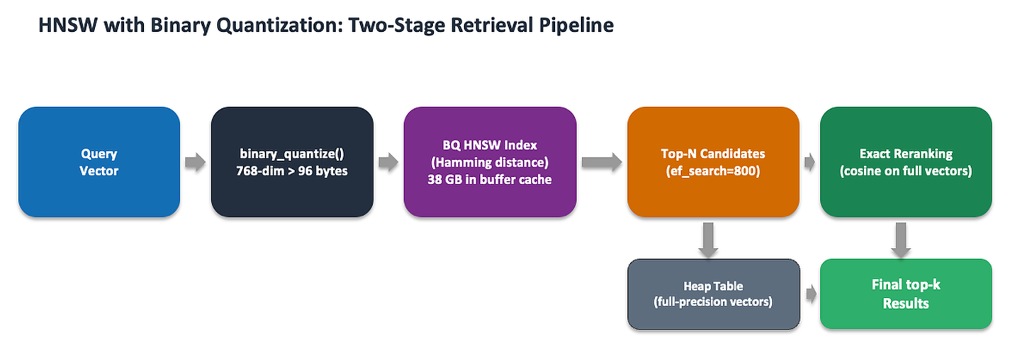
Figure 1: How HNSW with binary quantization and reranking works

We also evaluated a disk-based approximate nearest neighbor index approach. This approach uses statistical binary quantization (SBQ) for in-memory graph navigation and fetches full-precision vectors from disk for distance refinement. It follows the algorithmic approach described in Microsoft Research’s disk-based ANN research (MIT License). We refer to this approach as “disk-based ANN” throughout this post.

Benchmark setup

We tested on Aurora PostgreSQL 18.4 (pgvector 0.8.0) with Aurora I/O-Optimized storage using the following configuration:

• Instances: r8g.large (2 vCPUs, 16 GB RAM), r8g.4xlarge (16 vCPUs, 128 GB RAM), r8gd.4xlarge (16 vCPUs, 128 GB RAM, 950 GB NVMe), r8gd.12xlarge(48 vCPUs, 384 GB RAM, 1900 GB NVMe), r8g.48xlarge(192 vCPUs, 1.5 TB RAM)
• Datasets: LAION 100M (768-dim CLIP ViT-L/14 image embeddings), OpenAI 5M (1536-dim text-embedding-ada-002 text embeddings), Cohere 10M (768-dim embed-english-v3.0 text embeddings)
• Benchmark tool: VectorDBBench (open source, Zilliz) with top_k=100. recall@k values aren’t directly comparable across different k.
• Index Build Parameters:
  • HNSW (full precision), r8g.12xlarge, m=16, ef_construction=256, maintenance_work_mem=96GB, max_parallel_maintenance_workers=48.
  • HNSW+BQ (Hamming), r8g.12xlarge, m=16, ef_construction=256, maintenance_work_mem=96GB, max_parallel_maintenance_workers=48,quantization-type=bit.
  • Disk-based ANN (SBQ), r8g.48xlarge, num_neighbors = 50, search_list_size = 100, max_alpha = 1.2, num_bits_per_dimension = 2, diskann.force_parallel_workers=16 [>16 parallel workers impacted the recall quality], diskann.parallel_flush_interval = 0.05.
• Index Search Parameters:
  • HNSW, ef_search=256.
  • HNSW+BQ (LAION),ef_search=800,Rerank(qfl)=1400.
  • HNSW+BQ (OpenAI), ef_search=800,Rerank(qfl)=1400.
  • HNSW+BQ (Cohere), ef_search=800,Rerank(qfl)=1400.
  • Disk-based ANN (SBQ) (LAION), –query-search-list-size 200 –query-rescore 800.
• Client and methodology:
  • Benchmark tool: VectorDBBench v0.3.4 (open source, Zilliz) with top_k=100.
  • Client: c6i.16xlarge in the same AZ as the Aurora cluster.
  • Concurrency: ramped from 1 to 150 concurrent connections. Reported QPS is max sustained throughput.
  • Cold-start testing: instance type modifications flushed all caches between configurations; “cold” = first run after resize with no prior queries.

Note: We tested on Aurora PostgreSQL 18.4 in pre-release, but you can use any version specified in the prerequisites.

Performance characteristics across datasets

We compared full-precision HNSW, disk-based ANN (SBQ), and HNSW+BQ across three datasets and instance types. The following sections summarize the results for each.

OpenAI 5M (1536 dimensions) on r8g.large

On this memory-constrained instance, HNSW’s 38 GB index far exceeds the available 16 GB RAM, forcing disk I/O on every query and delivering only 78 QPS with 1,356ms p99 latency. Both HNSW+BQ and disk-based ANN produce compact 3.4 GB indexes (11.2x smaller) that fit entirely in the buffer cache.

Table 1

HNSW+BQ delivered 1.8x higher throughput than HNSW, 1.3x higher than disk-based ANN, with the best recall (0.951) and lowest latency (18.9ms p99). It also built 20x faster than disk-based ANN. The 1536-dimensional vectors produce high bit diversity under binary quantization, making the quantized index particularly effective at preserving neighbor relationships. Higher dimensionality gives BQ more bits to separate neighbors, though this is not guaranteed for all distributions, so validation remains essential.

Why BQ recall exceeds HNSW here (0.951 compared to 0.934): The BQ reranking step fetches 800 candidates and rescores them using exact cosine distance against full-precision vectors. This broader candidate pool (800) compared to HNSW’s graph traversal depth (ef_search=256) allows exact rescoring to surface neighbors that HNSW’s greedy traversal missed.

LAION 100M (768 dimensions) on r8g.4xlarge

HNSW’s 367 GB index cannot fit in the 128 GB buffer cache. Under cold-cache conditions representative of production workloads with diverse queries, HNSW delivered only 3.4 QPS. HNSW+BQ’s 38 GB index (9.7x smaller) and the disk-based ANN index’s 66 GB index both fit in cache.

Table 2

Cold-cache conditions represent the realistic production scenario for diverse queries. Under these conditions, HNSW+BQ delivered 4x higher throughput than HNSW and 1.8x higher than disk-based ANN. At high concurrency after cache warming, HNSW eventually reached 3,336 QPS because of benchmark query reuse warming the large index into cache. HNSW+BQ built in 1.1 hours compared to 31.5 hours for disk-based ANN (28.6x faster) and produced the smallest index footprint. The cold-cache column represents the first queries after a fresh instance start with no data in the buffer cache. The warm column represents steady state after repeated queries have populated the cache. Which column matters for your workload depends on your query distribution.

Cohere 10M (768 dimensions), the failure mode

This dataset exposed the limitations of all quantization-based methods. Disk-based ANN achieved a maximum recall of only 0.77, well below production requirements. HNSW+BQ was the only method to reach 0.93 recall. However, it required reranking 3,000 candidates per query using pgvector 0.8.0 iterative scans, collapsing throughput to 16 QPS with 1,640ms p99 latency. On a larger instance (r8g.12xlarge, 384 GB RAM) where the full HNSW index fits in memory, standard HNSW delivered 6,930 QPS at 0.952 recall. Quantization struggles with the clustered embedding distribution in this dataset.

Why quantization fails on this dataset: binary_quantize() thresholds each dimension at zero. The Cohere embed-english-v3.0 embeddings have a clustered distribution where many dimensions are concentrated near zero without balanced positive/negative spread. This means the sign bit carries little discriminative information, and many distinct vectors map to the same (or similar) bit patterns.

Sizing guidance: how many vectors can you store?

HNSW+BQ performance is determined by whether the quantized index fits in the PostgreSQL buffer cache. The index size is predictable: approximately 400 bytes per vector at 768 dimensions and 680 bytes per vector at 1536 dimensions. These 400 and 680 bytes figures are empirical at m=16. The neighbor-list overhead scales with the HNSW m parameter, so builds with m=24 or m=32 will produce larger indexes. The sizing rule for high query performance: Size your instance so that the BQ index occupies no more than 50–60% of shared_buffers, leaving the remaining buffer cache available for heap and TOAST pages fetched during reranking.

Table 3

With the BQ index memory-resident and qfl=1400 on LAION 100M, we measured approximately 50 QPS per vCPU (range: 47–56 across instances). This was measured on r8g.4xlarge (16 vCPU → 895 QPS, 55.9 QPS/vCPU) and r8g.12xlarge (48 vCPU → 2,261 QPS, 47.1 QPS/vCPU). On r8g.48xlarge, this projects to 9,000-10,000 QPS. The projection to 192 vCPUs (r8g.48xlarge → ~9,000–10,000 QPS) assumes linear scaling continues without connection pooling, lock contention, or NUMA bottlenecks becoming the constraint. For pricing, see Amazon Aurora pricing.

For customers whose vector counts exceed 2 billion, beyond what can fit in buffer cache even on the largest instances, NVMe-backed instances (r8gd family) remain a strong option. With Aurora I/O-Optimized (unlike on Standard clusters), the BQ index spills from buffer cache into the NVMe tier, which provides up to 4.6x higher throughput [LAION 100M dataset on r8gd.large, see Table 5] than non-NVMe (r8g.large) instances when the index (38 GB) exceeds available memory (16 GB). On r8gd.48xlarge, 2x instance memory reserved for temp objects, ~10% for internal operations, remainder is tiered cache (~7.3 TB on r8gd.48xlarge). At this capacity, the theoretical maximum vector capacity is approximately 20 billion vectors at 768-dim, 16 billion at 1024-dim, and 11.5 billion at 1536-dim. These estimates are empirical at m=16. The neighbor-list overhead scales with the HNSW ‘m’ parameter, so builds with m=24 or m=32 will produce larger indexes and reduce the effective vector ceiling accordingly. Query latencies will be higher compared to when the index fits completely in memory, but queries remain functional and recall is preserved, making NVMe-backed instances a viable architecture for workloads that would otherwise require complex sharding or partitioning strategies at these scales.

Caveats on the 20-billion-vector ceiling: The 20B figure is a theoretical maximum based on available NVMe storage capacity. Our largest measured run is 100 million vectors. Several PostgreSQL hard limits require partitioning well before 20B on a single table:

• 32 TB per relation: 20B vectors at 768-dim with TOASTed storage produces approximately 61 TB in the TOAST relation alone, exceeding the single-relation limit.
• 32-bit TOAST chunk OIDs: Approximately 4 billion out-of-line values maximum per table.
• Rerank heap fetches at this scale mostly miss both buffer cache and NVMe tiered cache, hitting Aurora storage with higher latency.

Partitioning is mandatory at billion-plus scale. What the NVMe architecture avoids is cross-database sharding. Table partitioning within a single Aurora cluster remains necessary. Query latencies will be higher compared to when the index fits completely in memory, but queries remain functional and recall is preserved.

Table 4

Table 5

For customers who need to scale beyond these vector limits, you can explore using Amazon S3 Vectors, a capability of Amazon S3, with Aurora PostgreSQL for cost-efficient tiered vector storage, keeping hot embeddings in Aurora for low-latency access while archiving cold vectors at S3 pricing. For implementation details, refer to Query billion-scale vectors with SQL: Integrating Amazon S3 Vectors and Aurora PostgreSQL.

When to use each approach

The right indexing strategy depends on your dataset size relative to available memory, your embedding characteristics, and your recall requirements.

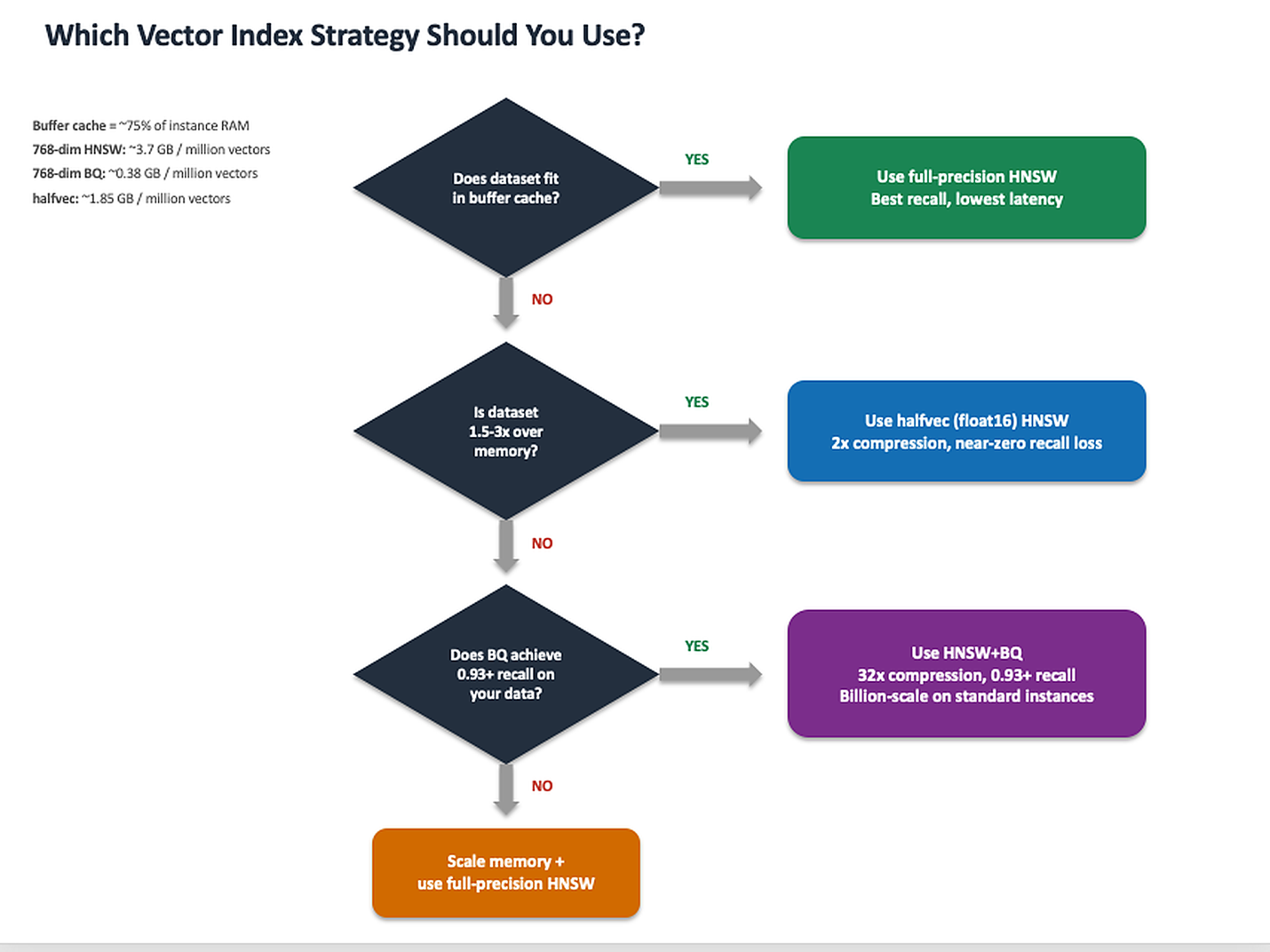
Figure 2: Choosing an indexing approach based on dataset size, embeddings, and recall requirements

Choose full-precision HNSW when your dataset fits in the instance buffer cache. At 768 dimensions, a full-precision HNSW index consumes approximately 3.7 GB per million vectors (367 GB / 100M). This means approximately 26 million vectors fit in an r8g.4xlarge (~96 GB buffer cache) and approximately 50 million vectors require an r8g.8xlarge (~192 GB buffer cache). If you need the absolute highest recall (0.96+) with the lowest possible latency and your workload has consistent query patterns that benefit from cache warming, there is no reason to introduce quantization overhead. HNSW delivers the best raw performance when memory is not the constraint.

Choose halfvec (float16 HNSW) as a low-risk middle step before binary quantization. The halfvec type stores vectors at half precision (2 bytes per dimension instead of 4), cutting index size by 2x with near-zero recall loss. This doubles your effective vector capacity within the same memory budget without the distribution-dependent risks of binary quantization. Consider halfvec when your dataset is 1.5–3x what fits in memory at full precision. It might avoid the need for BQ entirely.

-- halfvec: 2x compression with near-zero recall loss
CREATE INDEX idx_halfvec_hnsw ON your_table
USING hnsw ((embedding::halfvec(768)) halfvec_l2_ops)
WITH (m = 16, ef_construction = 256);

-- Query using halfvec index
SELECT id, embedding <-> '[query_vector]'::vector AS distance
FROM your_table
ORDER BY embedding::halfvec(768) <-> '[query_vector]'::halfvec(768)
LIMIT 10;

HNSW with binary quantization is our recommended approach for scale when your dataset exceeds available instance memory and you need hundred-million to billion-scale vector search. It works particularly well with:

• High-dimensional embeddings (1536+ dimensions) where bit diversity improves quantization effectiveness.
• Image-based embeddings (CLIP, LAION-style) at any dimension.
• Normalized embeddings (cosine similarity models) where dimensions are balanced around zero.

The approach delivers faster index builds than alternatives (1.1 hours compared to 31.5 hours at 100M scale), which is critical when embedding model upgrades require full reindexing. The prerequisite: validate recall meets your threshold (0.93+) on a representative sample of your actual data, because quantization effectiveness is distribution-dependent.

A disk-based ANN extension is worth considering if you are already using one on self-managed PostgreSQL and have validated recall on your specific dataset. Note: there are no disk-ANN extensions available on Aurora PostgreSQL or Amazon RDS for PostgreSQL. Under high-concurrency steady-state conditions, disk-based ANN converges with HNSW+BQ at approximately 900 QPS on 100M vectors. However, the tradeoffs are significant: index build times are 28x longer (31.5 hours for 100M vectors compared to 1.1 hours for HNSW+BQ), and index creation required an r8g.48xlarge (1.5 TB RAM) after OOM failures on smaller instances. These build-time and resource claims reflect our testing with the parameters documented in the Benchmark Setup section. Results might differ with alternative tuning.

Neither quantization method works well when your 768-dimension text embeddings have clustered distributions (as with Cohere embed-english-v3.0). If you require 0.95+ recall with sub-50 ms latency at 768 dimensions on text data, scale memory and use full-precision HNSW. On r8gd.12xlarge (384 GB), HNSW delivered 6,930 QPS at 0.952 recall on the same dataset where both quantization methods struggled.

Distance metric guidance

Binary quantization via Hamming distance approximates angular (cosine) similarity. When using HNSW+BQ:

• The index uses Hamming distance on the bit vectors (bit_hamming_ops)
• The rerank step must use your production distance metric: <=> (cosine), <-> (L2), or <#> (inner product)
• If your embeddings are not normalized, the sign-bit threshold at zero might not be meaningful. Consider normalizing before quantization.

Filtered queries

Post-filtering (for example, WHERE tenant_id = 'X') interacts poorly with ANN top-k: the index returns k candidates before filtering, so restrictive filters can eliminate most results. pgvector 0.8.0’s iterative scans (hnsw.iterative_scan = relaxed_order) address this by continuing to scan the index until enough post-filter results are found. For multi-tenant workloads with selective filters, iterative scans are essential. Set hnsw.max_scan_tuples high enough to accommodate your filter selectivity.

Getting started: implementing HNSW+BQ on Amazon Aurora PostgreSQL

Solution overview: The implementation follows a two-stage retrieval pattern: first, you build an HNSW index on binary-quantized vectors that fits in buffer cache at a fraction of the full-precision size. Then, at query time, you retrieve candidates using fast Hamming distance on the compressed index and rerank the top-N against full-precision vectors to recover accuracy. The steps below walk through index creation, query patterns with and without reranking, recall tuning, and validation against ground truth.

The first step is to create the binary quantized index on your table.

Step 1: Create the BQ index

-- Build parameters used in our 100M benchmark (1.1-hour build time) on instance type r8g.12xl
SET maintenance_work_mem = '96GB';
SET max_parallel_maintenance_workers = 48;

-- For 768-dim embeddings:
CREATE INDEX idx_bq_hamming ON your_table
USING hnsw ((binary_quantize(embedding)::bit(768)) bit_hamming_ops)
WITH (m = 16, ef_construction = 256);

-- For 1536-dim embeddings:
CREATE INDEX idx_bq_hamming ON your_table
USING hnsw ((binary_quantize(embedding)::bit(1536)) bit_hamming_ops)
WITH (m = 16, ef_construction = 256);

Step 2: Verify the index is used

EXPLAIN (COSTS OFF)
SELECT id FROM your_table
ORDER BY binary_quantize(embedding)::bit(768) <~> binary_quantize('[query_vector]'::vector)::bit(768)
LIMIT 10;

-- Expected output should show:
-- Index Scan using idx_bq_hamming on your_table
-- If you see "Seq Scan", the ORDER BY expression does not match the index expression.

Step 3: Query without reranking (fastest, lower recall)

SET hnsw.ef_search = 200;

SELECT id,
    binary_quantize(embedding)::bit(768) <~> binary_quantize('[query_vector]'::vector)::bit(768) AS hamming_dist
FROM your_table
ORDER BY binary_quantize(embedding)::bit(768) <~> binary_quantize('[query_vector]'::vector)::bit(768)
LIMIT 10;  -- k (top-k): final results returned to the caller

Step 4: Query with reranking (higher recall)

The inner query retrieves candidates from the BQ index. The outer query rescores them with exact distances. The LIMIT in the inner query is the quantized_fetch_limit (qfl) (how many candidates to rerank). The outer LIMIT is your top-k, the number of final nearest-neighbor results returned after exact-distance reranking.

Important: The HNSW index returns at most hnsw.ef_search candidates. You must set ef_search >= qfl, or for qfl > 1000, use iterative scans (pgvector 0.8.0+).

-- For qfl up to 1000: raise ef_search to match
SET hnsw.ef_search = 200;

SELECT * FROM (
    SELECT id, embedding <=> '[query_vector]'::vector AS exact_distance
    FROM your_table
    ORDER BY binary_quantize(embedding)::bit(768) <~> binary_quantize('[query_vector]'::vector)::bit(768)
    LIMIT 200 -- qfl=200, ef_search must be >= 200
) candidates
ORDER BY exact_distance
LIMIT 10;

Step 5: Tune recall by increasing reranking progressively

Start at 10–20x your top_k (so qfl=100–200 for top_k=10) and increase until recall meets your target:

-- Step A: qfl=200 (fastest, ef_search=200 sufficient)
SET hnsw.ef_search = 200;
SELECT * FROM (
    SELECT id, embedding <=> '[query_vector]'::vector AS exact_distance
    FROM your_table
    ORDER BY binary_quantize(embedding)::bit(768) <~> binary_quantize('[query_vector]'::vector)::bit(768)
    LIMIT 200
) candidates ORDER BY exact_distance LIMIT 10;

-- Step B: qfl=400 (raise ef_search to match)
SET hnsw.ef_search = 400;
SELECT * FROM (
    SELECT id, embedding <=> '[query_vector]'::vector AS exact_distance
    FROM your_table
    ORDER BY binary_quantize(embedding)::bit(768) <~> binary_quantize('[query_vector]'::vector)::bit(768)
    LIMIT 400
) candidates ORDER BY exact_distance LIMIT 10;

-- Step C: qfl=800 (raise ef_search to match)
SET hnsw.ef_search = 800;
SELECT * FROM (
    SELECT id, embedding <=> '[query_vector]'::vector AS exact_distance
    FROM your_table
    ORDER BY binary_quantize(embedding)::bit(768) <~> binary_quantize('[query_vector]'::vector)::bit(768)
    LIMIT 800
) candidates ORDER BY exact_distance LIMIT 10;

-- Step D: qfl=1400 (exceeds ef_search cap of 1000 -- use iterative scans)
SET hnsw.iterative_scan = relaxed_order;
SET hnsw.max_scan_tuples = 1400;
SET hnsw.ef_search = 1000; -- max allowed value
SELECT * FROM (
    SELECT id, embedding <=> '[query_vector]'::vector AS exact_distance
    FROM your_table
    ORDER BY binary_quantize(embedding)::bit(768) <~> binary_quantize('[query_vector]'::vector)::bit(768)
    LIMIT 1400
) candidates ORDER BY exact_distance LIMIT 10;

Step 6: Measure true recall (exact scan ground truth)

For accurate recall measurement, compare against brute-force exact search (not another approximate index):

-- Ground truth: disable index scan to force exact sequential scan
BEGIN;
SET LOCAL enable_indexscan = off;
SET LOCAL enable_bitmapscan = off;
SELECT id FROM your_table
ORDER BY embedding <=> '[query_vector]'::vector
LIMIT 10;
COMMIT;

Validation before production deployment

Before committing to HNSW+BQ in production, validate recall against ground truth on a representative sample of your actual data. Binary quantization effectiveness is distribution-dependent. It works well on some embedding models and fails on others. We recommend the following process:

1. Generate ground truth nearest neighbors for 1,000–10,000 representative queries using brute-force exact search (sequential scan with indexes disabled, as shown in Step 6 above).
2. Build an HNSW+BQ index on your dataset and measure recall@k at your target k value.
3. Tune quantized_fetch_limit (the reranking candidate count) starting at 10–20x your top_k. Each additional reranking candidate adds several page reads per query (heap + TOAST pages for the full-precision vector).
4. Measure throughput at your target concurrency level at the chosen qfl.
5. If recall does not reach your threshold at acceptable throughput, consider halfvec (float16) HNSW as a middle ground, or use full-precision HNSW with sufficient memory.

Operational considerations

Aurora read replicas scale QPS horizontally, each replica maintains its own buffer cache with the BQ index. After a failover, both buffer cache and NVMe tiered cache start cold. Our measurements show cold-start throughput at ~13.5 QPS compared to ~895 QPS warm on r8g.4xlarge with LAION 100M. Plan for a warm-up period or use pg_prewarm to accelerate recovery.

Clean up resources

If you created indexes or test tables while following this post, remove them to avoid unnecessary storage costs:

-- Drop the binary quantized index
DROP INDEX IF EXISTS idx_bq_hamming;

-- If you created a dedicated test table for validation
DROP TABLE IF EXISTS your_test_table;

If you provisioned a larger Aurora instance specifically for benchmarking, scale it back down to your production instance size or delete the cluster if it was created solely for testing. You can modify the instance class from the Amazon RDS console or using the AWS Command Line Interface (AWS CLI):

aws rds modify-db-instance --db-instance-identifier your-instance --db-instance-class db.r8g.xlarge --apply-immediately

Conclusion

In this post, we showed how HNSW with binary quantization delivers hundred-million to billion-scale vector search on Aurora PostgreSQL without additional extensions, with faster index builds, smaller footprints, and equal or better query performance compared to disk-based ANN alternatives on the datasets we tested. It is the recommended path for customers outgrowing standard HNSW’s memory requirements.

The key tradeoffs to understand:

Reranking cost: Each query fetches original vectors from the heap table for the top-N candidates (3–4 page reads per candidate because of TOAST), so throughput is sensitive to buffer cache state and the number of candidates reranked.

Distribution dependency: Not all embedding models produce vectors that quantize well. Validate on your data before committing.

Scaling limits: Single-table PostgreSQL limits (32 TB, TOAST OIDs) require partitioning at billion-plus scale.

For workloads where quantization does not validate, halfvec (float16) HNSW offers a 2x compression middle ground, and full-precision HNSW with sufficient memory remains the correct answer when recall is paramount.

pgvector binary quantization support is available today on Aurora PostgreSQL and RDS for PostgreSQL. For more information, refer to the pgvector GitHub repository and the Aurora PostgreSQL User Guide or RDS for PostgreSQL User Guide.

About the authors