Supply chain data analysis and visualization using Amazon Neptune and the Neptune workbench

Many global corporations are managing multiple supply chains, and they depend on those operations to not only deliver goods on time but to respond to divergent customer and supplier needs. According to a McKinsey study, it’s estimated that significant disruptions to production now occur every 3.7 years on average, adding new urgency to supply chain resiliency questions for CEOs, boards of directors, and investors—not just operational leaders. Additionally, the study found that as much as 45% of one year’s earnings could be lost each decade because of supply chain disruptions. Therefore, with full supply chain visibility, you can gather information about your supply chain network and store it in a database that gives you end-to-end control, providing advantages like increased visibility, bottleneck identification, and in-depth understanding of the suppliers.

Relational databases aren’t optimized for very complex queries that involve multiple joins or when frequent schema changes are required. Graph databases, on the other hand, can make data correlations based on graphs and are ideal for organizing and visualizing this data as an integrated whole because they directly represent the network. Graph analytics on Amazon Neptune of highly connected supply chain data gives you the tools to ask deep and complex questions that understand not only the individual data points, but the relationships between all the cooperating links in the chain.

In this post, we show how you can use a Neptune graph database to visualize interrelationships of a supply chain using the Neptune workbench, which lets you quickly and easily query Amazon Neptune databases with Jupyter notebooks in a fully managed, interactive development environment with live code and narrative text, and identify all direct and indirect neighbors of a product, component, or supplier.

Overview of solution

For this post, we consider a fictitious automotive manufacturing company that builds various car types and models. We go through how to visualize and analyze the supply chain for this company for various use cases using Neptune through the Neptune workbench using the Gremlin query language.

The following diagram provides a high-level overview of how the various components of this fictitious car manufacturing company are related to each other. This provides an overview how the supplier organization and subsidiaries are related with the company, the locations where the factories and warehouses are operating, the various products required to build the car, and how they’re related to demand.

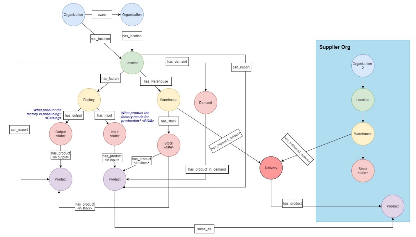
Figure-1: Overall Flow

Generally, a car manufacturing company might have the following different data types:

Organizational data containing documentation, processes, facilities, hierarchies, systems and databases, and more
Product data containing product details or bill of materials (BoM)
Customer data containing CRM, corporate data, and so on
Third-party data like dealer data, social media, and market data
Event data like telematics data, customer connect, or warranty information
Supply chain data like supplier data, inventory data, or logistics data

For this post, we use data related to inventory, BoM, facilities, and hierarchies.

Prerequisites

For this walkthrough, you should have the following prerequisites:

An AWS account.
A Neptune database cluster and Amazon SageMaker notebook (Neptune workbench).
Knowledge of Gremlin and Jupyter notebooks.
An AWS Identity and Access Manager (IAM) user with the permissions you need for working with your Neptune DB cluster. For more information, refer to Creating an IAM user with permissions for Neptune.

For this post, we use Region us-east-1. Also, note that customer is responsible for the costs of the resources for this post.

Create solution resources

The easiest way to create a new Neptune DB cluster and the various resources for this post is to use an AWS CloudFormation template, which creates all the required resources for you, without having to do everything by hand. To launch a new provisioned Neptune DB cluster, complete the following steps:

Launch the CloudFormation stack in us-east-1, choosing Launch Stack (this CloudFormation template is available in the GitHub repo).

Using the default configurations in the stack, estimated approximate cost is $1 per day, with the assumption that the cluster and the notebook instance will be running for 1 hour. Pricing details are available in Amazon Neptune pricing page.

Provide a stack name (for example, DemoNeptuneStack).
For AttachBulkloadIAMRoleToNeptuneCluster, choose false.
Keep the default values for DBClusterPort, DBReplicaIdentifierSuffix, and DbInstanceType.

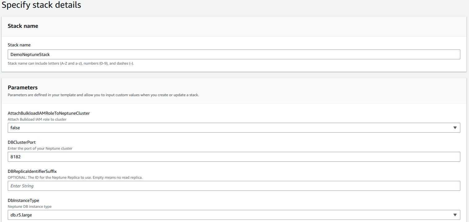
Figure-2: CloudFormation Stack Details

For ENV, enter demoscmblog.
Keep the default values for IamAuthEnabled, NeptuneEnableAuditLog, NeptuneQueryTimeout, and NeptuneSagemakerNotebookStartupScript.
For NotebookInstanceType, choose ml.t3.xlarge.

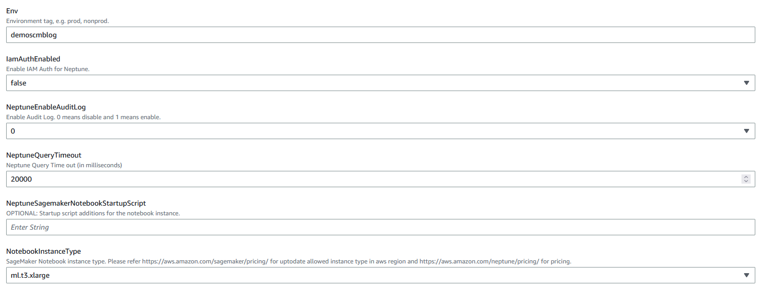
Figure-3: CloudFormation Stack Details

Complete the stack creation. Stack takes ~15 – 20 minutes to complete.
When the template is complete, navigate to the Outputs tab for the stack to get the details of the resources you created.

Verify the Neptune cluster and workbench

To verify the Neptune cluster and workbench, complete the following steps:

On the Neptune console, choose Databases in the navigation pane.

This page shows the Neptune cluster details. The cluster should be in the Available state.

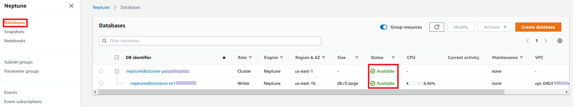
Figure-4: Neptune cluster state

Choose Notebooks in the navigation pane to get the details of the notebook attached with the Neptune cluster.

The notebook must be in the Ready state.

Select the notebook and on the Actions menu, choose Open Jupyter.

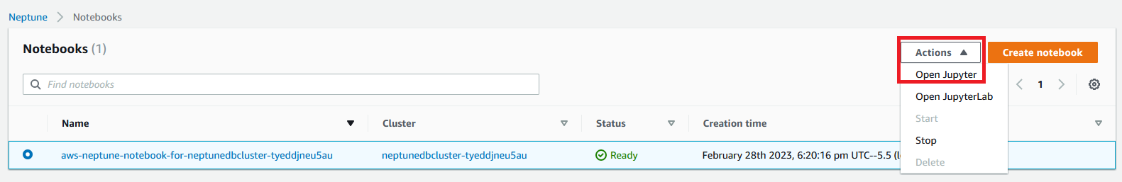
Figure-5: Open Jupyter

Create a Jupyter notebook

To create a Jupyter notebook, complete the following steps:

Open the notebook and choose the folder Neptune.

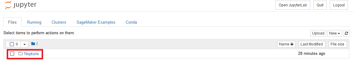
Figure-6: Open Neptune Folder

Inside the Neptune folder, there are some pre-created folders with sample notebooks.

Create a folder named DemoSCMBlog.

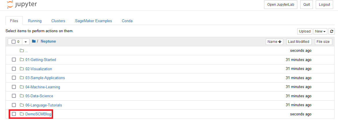
Figure-7: Create Folder

Navigate inside the DemoSCMBlog folder, choose New, and choose Python 3 to create an IPYNB file with Python 3 and a Neptune kernel.

This opens a new tab in the browser.

Rename the file DemoDataAnalysis.

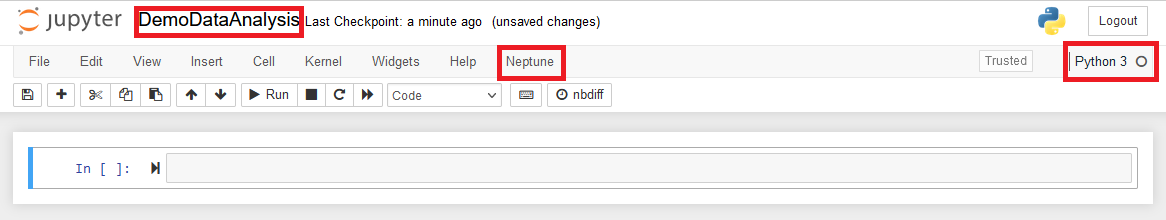
Figure-8: Create Notebook

This notebook is available for download on the GitHub repo. This notebook can also be imported into the instance by clicking on the Upload button Jupyter.

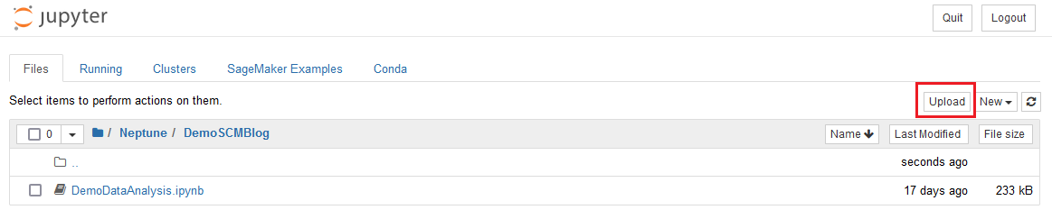
Figure-9: Upload Notebook

Create the data

In this section, we create the fictitious data required for analysis. We use Gremlin magic (%%gremlin) for this post. For more information, refer to Using Neptune workbench magics in your notebooks. Note that a key component of working with graph databases is the corresponding data model. For more details, refer to Neptune Graph Data Model.

In this section, we create the following:

Seven companies with names as TestCo-*.
Various facilities, warehouses, and factories required for the analysis. We consider various types of cars like sedans and roadsters, and various components of the car like the front seat, rear seat, heating, springs, steel, and more.

Complete the following steps to create the sample data:

Create the various companies, suppliers, and subsidiaries:

%%gremlin
// create locations, suppliers, subsidiaries
g.addV('company').
  property(id, 'company-1').
  property('name', 'TestCo-1').
  addV('company').
  property(id, 'company-2').
  property('name', 'TestCo-2').
  addV('company').
  property(id, 'company-3').
  property('name', 'TestCo-3').
  addV('company').
  property(id, 'company-4').
  property('name', 'TestCo-4').
  addV('company').
  property(id, 'company-5').
  property('name', 'TestCo-5').
  addV('company').
  property(id, 'company-6').
  property('name', 'TestCo-6').
  addV('company').
  property(id, 'company-7').
  property('name', 'TestCo-7').
  next()

Add the locations, warehouses, factories, products, and stock information:

%%gremlin

//add locations, warehouses, factories, products, stocks

g
    // locations
    .addV('location').property(id, 'company-2-location-1').property('name', 'Facility-1')
    .addV('location').property(id, 'company-2-location-2').property('name', 'Facility-2')
    .addV('location').property(id, 'company-5-location-1').property('name', 'Facility-3')
    .addV('location').property(id, 'company-5-location-2').property('name', 'Facility-4')
    .addV('location').property(id, 'company-6-location-1').property('name', 'Facility-5')
    .addV('location').property(id, 'company-7-location-1').property('name', 'Facility-6')

    // warehouses
    .addV('warehouse').property(id, 'company-2-location-1-warehouse').property('name', 'Warehouse-1')
    .addV('warehouse').property(id, 'company-2-location-2-warehouse').property('name', 'Warehouse-2')
    .addV('warehouse').property(id, 'company-5-location-1-warehouse').property('name', 'Warehouse-3')
    .addV('warehouse').property(id, 'company-5-location-2-warehouse').property('name', 'Warehouse-4')
    .addV('warehouse').property(id, 'company-6-location-1-warehouse').property('name', 'Warehouse-5')
    .addV('warehouse').property(id, 'company-7-location-1-warehouse').property('name', 'Warehouse-6')

    // factories
    .addV('factory').property(id, 'company-2-location-1-factory').property('name', 'Factory-1')
    .addV('factory').property(id, 'company-2-location-2-factory').property('name', 'Factory-2')
    .addV('factory').property(id, 'company-5-location-1-factory').property('name', 'Factory-3')
    .addV('factory').property(id, 'company-5-location-2-factory').property('name', 'Factory-4')
    .addV('factory').property(id, 'company-6-location-1-factory').property('name', 'Factory-5')
    .addV('factory').property(id, 'company-7-location-1-factory').property('name', 'Factory-6')

    // products
    .addV('product').property(id, 'company-2-product-1').property('name', 'Sedan Car')
    .addV('product').property(id, 'company-2-product-2').property('name', 'SUV Car')
    .addV('product').property(id, 'company-5-product-1').property('name', 'Front Seat')
    .addV('product').property(id, 'company-5-product-2').property('name', 'Rear Seat')
    .addV('product').property(id, 'company-5-product-3').property('name', 'Bench Seat')
    .addV('product').property(id, 'company-6-product-1').property('name', 'Springs')
    .addV('product').property(id, 'company-6-product-2').property('name', 'Heating')
    .addV('product').property(id, 'company-7-product-1').property('name', 'Steel')

    // stocks
    .addV('stock').property(id, 'company-2-location-1-warehouse-stock-1').property('date', datetime('2022-08-01'))
    .addV('stock').property(id, 'company-2-location-1-warehouse-stock-2').property('date', datetime('2022-08-02'))
    .addV('stock').property(id, 'company-7-location-1-warehouse-stock-1').property('date', datetime('2022-08-01'))
    .addV('stock').property(id, 'company-7-location-1-warehouse-stock-2').property('date', datetime('2022-08-02'))
    .next()

Verify the number of companies created (it should be seven):

%%gremlin

// check number of companies
g.V().hasLabel('company').count()

Verify the total number of products created (it should be eight):

%%gremlin

// check the total number of products
g.V().hasLabel('product').count()

Add relationships in the data

In this section, we start creating the relationships among the different nodes to create the supply chain network for the automotive company.

Add the company ownership structure

We want to add the company ownership structure. To do that, we need to create an edge and connect a company with its subsidiaries. Here we add an edge of type owns, which connects the companies as per the ownership structure. This essentially notes that a company owns or is related with another company. See the following code:

%%gremlin

g.addE('owns').from(__.V('company-1')).to(__.V('company-2')).
  addE('owns').from(__.V('company-1')).to(__.V('company-3')).
  addE('owns').from(__.V('company-4')).to(__.V('company-5')).
  next()

The preceding query creates an ownership structure between the companies, where TestCo-1 owns TestCo-2 and TestCo-3, and TestCo-4 owns TestCo-5. Let’s now visualize this construct in the workbench using the following query:

%%gremlin -p v,oute,inv

g.V().outE().inV().path().by('name').by(label())

This query creates the following graphical depiction on the Graph tab in the output.

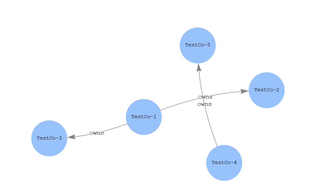
Figure-10: Company ownership

Create relationships between factories, warehouses, products, and stock

To create the supply chain graph for the fictitious automotive company, we create relationships between the following:

Companies connecting to locations (facilities)
Locations connecting to the warehouses
Locations connecting to the factories
Companies containing products in their catalog
Relationships between products, depicting their materials, quantities, and so on
Stock of the products in the warehouses at different dates
Relationship between the products and the stock

Use the following queries to create these relationships:

%%gremlin

g.addE('has_location').
    from(__.V('company-2')).
    to(__.V('company-2-location-1')).
  addE('has_location').
    from(__.V('company-2')).
    to(__.V('company-2-location-2')).
  addE('has_location').
    from(__.V('company-5')).
    to(__.V('company-5-location-1')).
  addE('has_location').
    from(__.V('company-5')).
    to(__.V('company-5-location-2')).
  addE('has_location').
    from(__.V('company-6')).
    to(__.V('company-6-location-1')).
  addE('has_location').
    from(__.V('company-7')).
    to(__.V('company-7-location-1')).
  addE('has_warehouse').
    from(__.V('company-2-location-1')).
    to(__.V('company-2-location-1-warehouse')).
  addE('has_warehouse').
    from(__.V('company-2-location-2')).
    to(__.V('company-2-location-2-warehouse')).
  addE('has_warehouse').
    from(__.V('company-5-location-1')).
    to(__.V('company-5-location-1-warehouse')).
  addE('has_warehouse').
    from(__.V('company-5-location-2')).
    to(__.V('company-5-location-2-warehouse')).
  addE('has_warehouse').
    from(__.V('company-6-location-1')).
    to(__.V('company-6-location-1-warehouse')).
  addE('has_warehouse').
    from(__.V('company-7-location-1')).
    to(__.V('company-7-location-1-warehouse')).
  addE('has_factory').
    from(__.V('company-2-location-1')).
    to(__.V('company-2-location-1-factory')).
  addE('has_factory').
    from(__.V('company-2-location-2')).
    to(__.V('company-2-location-2-factory')).
  addE('has_factory').
    from(__.V('company-5-location-1')).
    to(__.V('company-5-location-1-factory')).
  addE('has_factory').
    from(__.V('company-5-location-2')).
    to(__.V('company-5-location-2-factory')).
  addE('has_factory').
    from(__.V('company-6-location-1')).
    to(__.V('company-6-location-1-factory')).
  addE('has_factory').
    from(__.V('company-7-location-1')).
    to(__.V('company-7-location-1-factory')).
  addE('has_in_catalog').
    from(__.V('company-2')).
    to(__.V('company-2-product-1')).
  addE('has_in_catalog').
    from(__.V('company-2')).
    to(__.V('company-2-product-2')).
  addE('has_in_catalog').
    from(__.V('company-5')).
    to(__.V('company-5-product-1')).
  addE('has_in_catalog').
    from(__.V('company-5')).
    to(__.V('company-5-product-2')).
  addE('has_in_catalog').
    from(__.V('company-5')).
    to(__.V('company-5-product-3')).
  addE('has_in_catalog').
    from(__.V('company-6')).
    to(__.V('company-6-product-1')).
  addE('has_in_catalog').
    from(__.V('company-6')).
    to(__.V('company-6-product-2')).
  addE('has_in_catalog').
    from(__.V('company-7')).
    to(__.V('company-7-product-1')).
  addE('made_of').
    from(__.V('company-2-product-1')).
    to(__.V('company-5-product-1')).
  property('unit', 'PC').
  property('qty', 2).
  addE('made_of').
    from(__.V('company-2-product-2')).
    to(__.V('company-5-product-1')).
  property('unit', 'PC').
  property('qty', 2).
  addE('made_of').
    from(__.V('company-2-product-1')).
    to(__.V('company-7-product-1')).
  property('unit', 'KG').
  property('qty', 123.45).
  addE('made_of').
    from(__.V('company-2-product-2')).
    to(__.V('company-5-product-1')).
  property('unit', 'KG').
  property('qty', 123.45).
  addE('made_of').
    from(__.V('company-2-product-1')).
    to(__.V('company-5-product-2')).
  property('unit', 'PC').
  property('qty', 3).
  addE('made_of').
    from(__.V('company-2-product-2')).
    to(__.V('company-5-product-2')).
  property('unit', 'PC').
  property('qty', 3).
  addE('made_of').
    from(__.V('company-2-product-2')).
    to(__.V('company-5-product-3')).
  property('unit', 'PC').
  property('qty', 2).
  addE('made_of').
    from(__.V('company-5-product-1')).
    to(__.V('company-6-product-1')).
  property('unit', 'PC').
  property('qty', 1).
  addE('made_of').
    from(__.V('company-5-product-2')).
    to(__.V('company-6-product-1')).
  property('unit', 'PC').
  property('qty', 1).
  addE('made_of').
    from(__.V('company-5-product-3')).
    to(__.V('company-6-product-1')).
  property('unit', 'PC').
  property('qty', 1).
  addE('made_of').
    from(__.V('company-5-product-1')).
    to(__.V('company-6-product-2')).
  property('unit', 'PC').
  property('qty', 1).
  addE('made_of').
    from(__.V('company-5-product-2')).
    to(__.V('company-6-product-2')).
  property('unit', 'PC').
  property('qty', 1).
  addE('made_of').
    from(__.V('company-5-product-3')).
    to(__.V('company-6-product-2')).
  property('unit', 'PC').
  property('qty', 1).
  addE('made_of').
    from(__.V('company-6-product-1')).
    to(__.V('company-7-product-1')).
  property('unit', 'KG').
  property('qty', 0.12).
  addE('made_of').
    from(__.V('company-6-product-2')).
    to(__.V('company-7-product-1')).
  property('unit', 'KG').
  property('qty', 3.4).
  addE('has_stock').
    from(__.V('company-2-location-1-warehouse')).
    to(__.V('company-2-location-1-warehouse-stock-1')).
  property('date', datetime('2022-08-01')).
  addE('has_stock').
    from(__.V('company-2-location-1-warehouse')).
    to(__.V('company-2-location-1-warehouse-stock-2')).
  property('date', datetime('2022-08-02')).
  addE('has_stock').
    from(__.V('company-7-location-1-warehouse')).
    to(__.V('company-7-location-1-warehouse-stock-1')).
  property('date', datetime('2022-08-01')).
  addE('has_stock').
    from(__.V('company-7-location-1-warehouse')).
    to(__.V('company-7-location-1-warehouse-stock-2')).
  property('date', datetime('2022-08-02')).
  addE('has_product_in_stock').
    from(__.V('company-2-location-1-warehouse-stock-1')).
    to(__.V('company-2-product-1')).
  property('unit', 'PC').
  property('qty', 10).
  property('date', datetime('2022-08-01')).
  addE('has_product_in_stock').
    from(__.V('company-2-location-1-warehouse-stock-1')).
    to(__.V('company-2-product-2')).
  property('unit', 'PC').
  property('qty', 4).
  property('date', datetime('2022-08-01')).
  addE('has_product_in_stock').
    from(__.V('company-2-location-1-warehouse-stock-2')).
    to(__.V('company-2-product-1')).
  property('unit', 'PC').
  property('qty', 2).
  property('date', datetime('2022-08-02')).
  addE('has_product_in_stock').
    from(__.V('company-2-location-1-warehouse-stock-2')).
    to(__.V('company-2-product-2')).
  property('unit', 'PC').
  property('qty', 0).
  property('date', datetime('2022-08-02')).
  addE('has_product_in_stock').
    from(__.V('company-7-location-1-warehouse-stock-1')).
    to(__.V('company-7-product-1')).
  property('unit', 'KG').
  property('qty', 123.45).
  property('date', datetime('2022-08-01')).
  addE('has_product_in_stock').
    from(__.V('company-7-location-1-warehouse-stock-2')).
    to(__.V('company-7-product-1')).
  property('unit', 'KG').
  property('qty', 0).
  property('date', datetime('2022-08-02'))

Visualize the overall graph

Now let’s visualize the overall graph and the various connectivity between the elements in this supply chain. Here we get the connectivity between the following:

A company (for example TestCo-6) has locations of the facility, and that location has a warehouse and factory.
A catalog of products connecting to the company. These products are made of other products, which in turn are catalogs of other companies.

The following query shows the connectivity graph for this use case:

%%gremlin -p v,oute,inv

g.V().outE().inV().path().by(elementMap())

The query yields the following graph, which shows the overall connectivity for this supply chain.

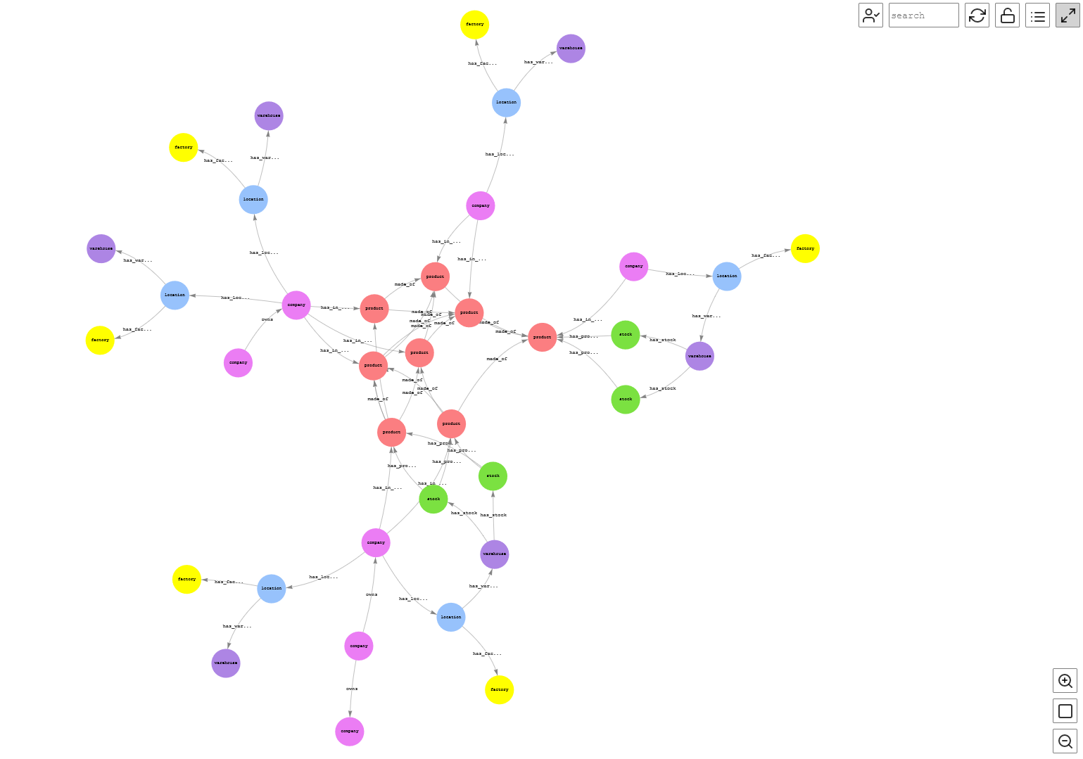
Figure-11: Complete Graph

Graph traversal for key KPIs

In this section, we traverse the supply chain graph for the fictitious automotive company created in the preceding sections and start to get some actionable KPIs. We’re interested in the following:

The bill of materials for a car
The various components the car is made of
The stock for a certain car type in all the warehouses

Find the BOM for a car

A key component is to get the bill of materials (BOM) for a certain product. It can define products as they are designed, as they are ordered, as they are built, or as they are maintained. This is essentially a recipe of the product. So, for example, to get the BOM of a car for this post, we run the following query over the sample data. In this example, we’re looking into the BOM for a sedan car, what that car is made of (like seats and steel), and the corresponding available quantity. This query traverses the created graph to get the details for a certain product.

%%gremlin -p v,oute,inv,oute,inv,oute,inv,oute,inv

// get BoM

g.V().
  has('name', 'Sedan Car').as('product').
  outE('made_of').
  inV().as('material').
  path().by('name').by('qty')

The following is the graphical representation of the query available in the workbench. This graph shows that Sedan Car is made of components like Front Seat, Rear Seat, and Steel, and also shows the corresponding quantity of the components.

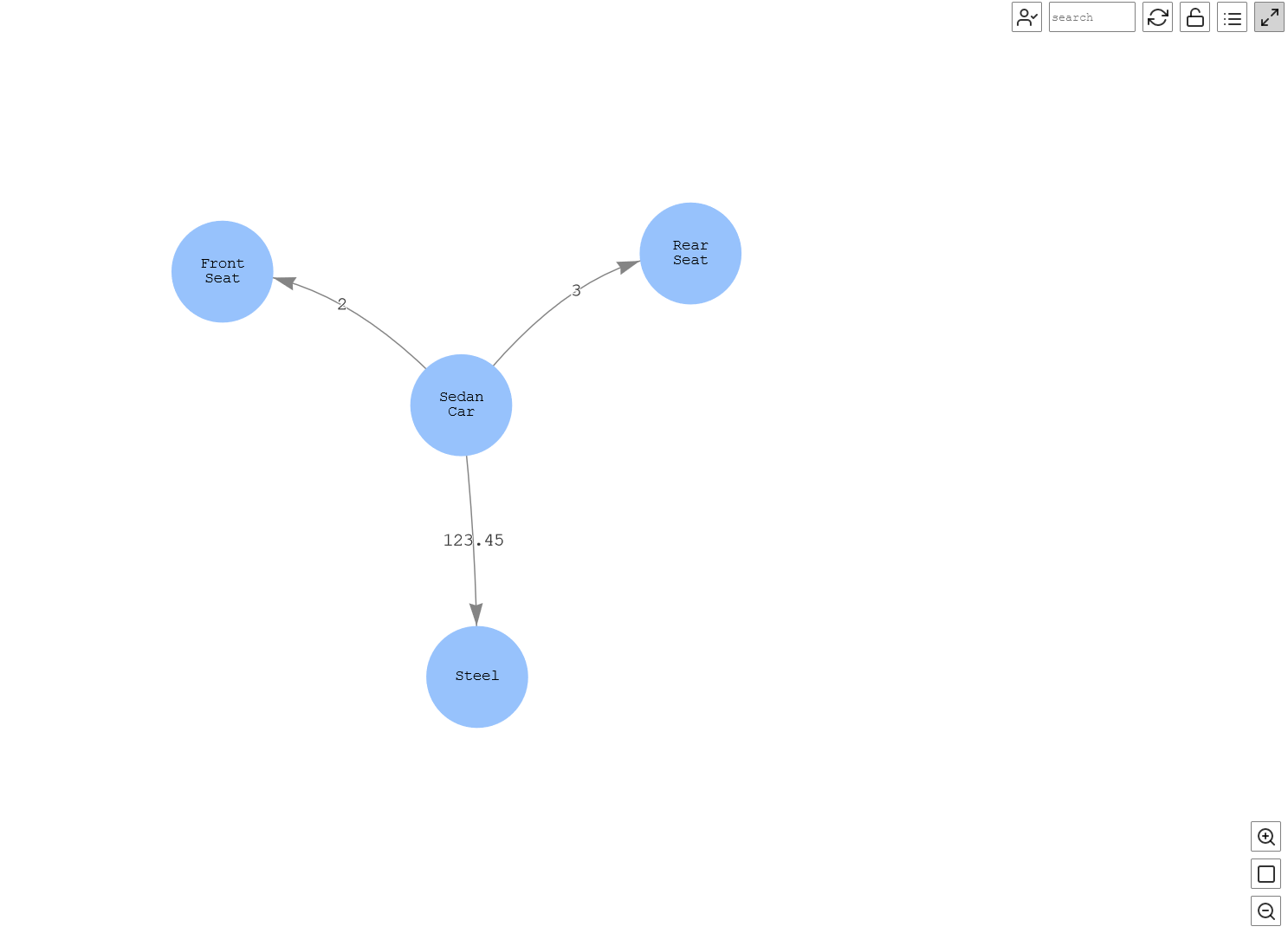
Figure-12: Bill of material

Find the various components that the car is made of

In this part of the analysis of the BOM, we want to know what the front seat of the car is made of and subsequently the material that those components are made of. This means that we want to check the linkages for a certain product at the nth level of depth, which is useful for analysis and taking required actions. In this case, Neptune adds the value in this use case where the nth level of information can be queried and analyzes the shortages, for example, which can impact the production.

In the following query, we query the car to get the details; for example, the rear seats are made of springs and heating components. The graph also shows that springs are made of steel, and this way you can query until the nth level of details of a complex relationship. In this example, times(2) has been added in the query, which essentially repeats the query twice, giving the second level of details. Note that we can change this number to any value to get the desired level of details. Therefore, through this example, you can determine the nth-level supplier for a customer.

%%gremlin -p v,oute,inv,oute,inv,oute,inv

// get the entire N tier supply

g.V().
  has('name', 'Sedan Car').as('product').
  outE('made_of').
  inV().as('material').
  optional(repeat(outE('made_of').inV().as('material')).times(2).emit()).
  path().by('name').by('qty')

Let’s visualize the query output.

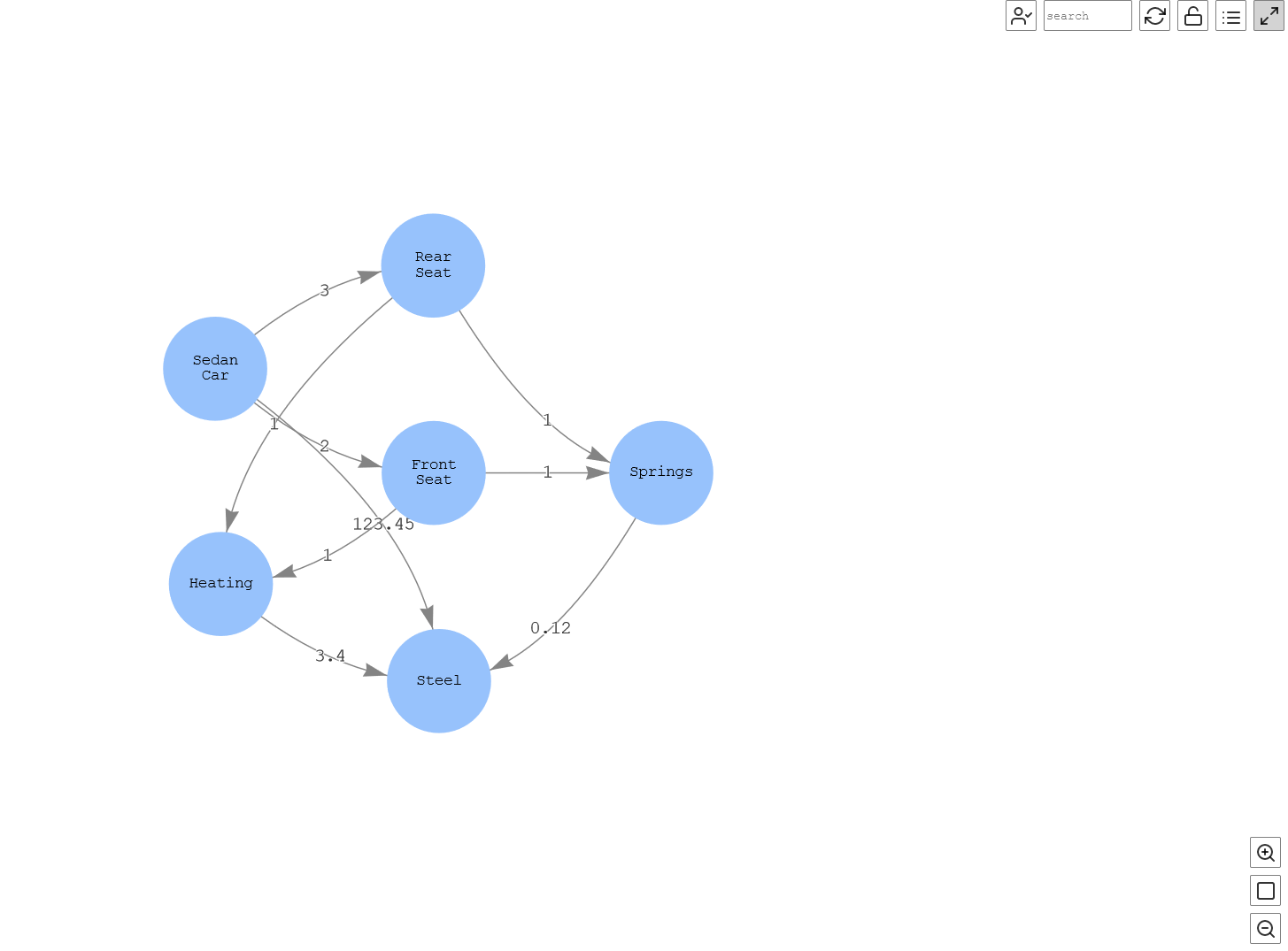
Figure-13: Various Components of a car

This graph shows that Sedan Car is made of Front Seat and Rear Seat, which have the component Heating, and both are made of Steel (the second-level details).

Find the stock for a certain car type in all the warehouses

Now let’s query the graph to understand the stock the company and its subsidiaries have in all the warehouses for Sedan Car so that any possible impact on the production can be handled.

In the following query, we can visualize that all the warehouses have total of 10 sedan cars as of August 1, 2022:

%%gremlin -p v,ine,outv

// get company's stock for a date
g.V().has('name', 'Sedan Car').as('product')
    .inE('has_product_in_stock').has('date', datetime('2022-08-01')).outV().as('stock')
    .path().by('name').by('qty').by('date')

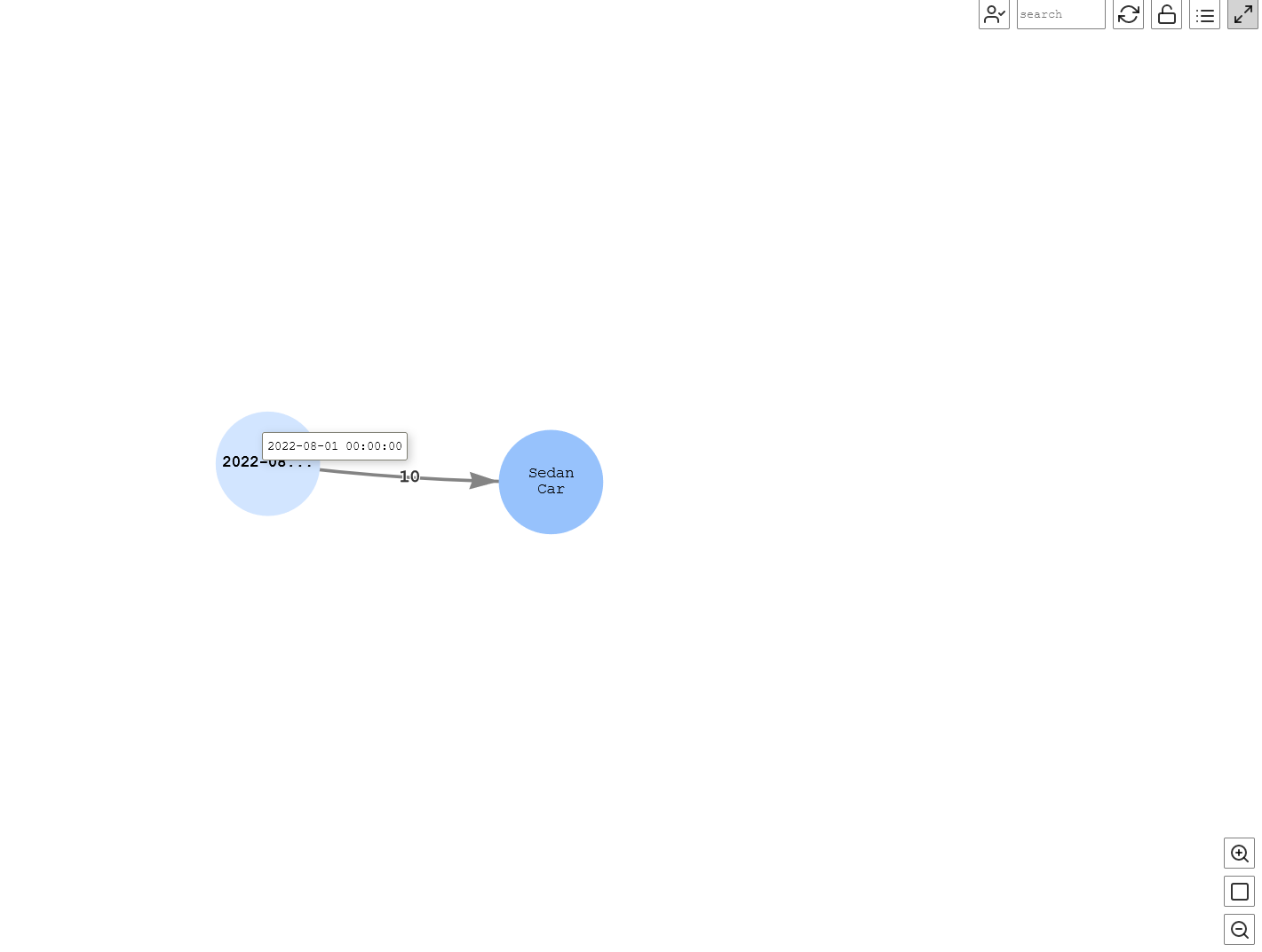
Figure-14: Stock at a date

As an automotive organization, we want to know all the stock that our subsidiaries have. To do that, the following query traverses the graph for TestCo-1 to get the details of the stock, including the subsidiaries, as of August 1, 2022:

%%gremlin -p v,oute,inv,oute,inv,oute,inv,oute,inv,oute,inv

// get the stock from all the subsidiaries for a given date
g.V().
  has('name', 'TestCo-1').
  outE('owns').
  inV().as('subsidiary').
  optional(
    outE('has_location').
    inV().as('location').
    outE('has_warehouse').
    inV().as('warehouse').
    optional(
      outE('has_stock').
      has('date', datetime('2022-08-01')).
      inV().as('stock').
      outE('has_product_in_stock').
      inV().as('product'))).
  path().by(elementMap())

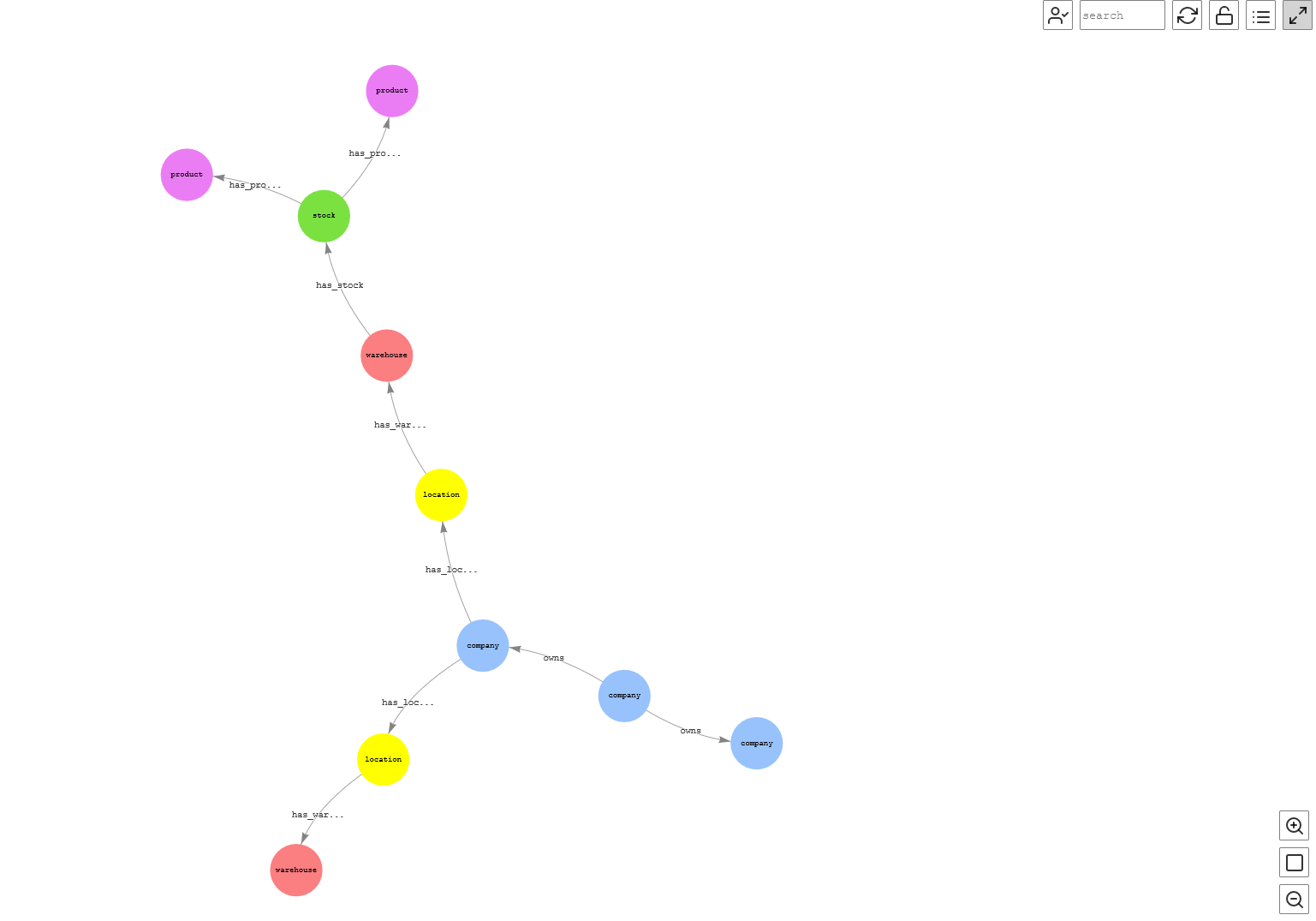
Figure-15: Stock for a company and subsidiaries

This visualization provides the details that TestCo-2, which is a subsidiary of TestCo-1 (owned by TestCo-1), has Facility-1, which constitutes of Warehouse-1, and on August 1, 2022, it had stock for Sedan Car and Roadster Car.

Another crucial use case could be to know all the stock in the supply chain for a certain product and its corresponding components at a certain date. This provides the critical information for any corrective actions to be taken so that shortage of stock can be avoided. See the following query:

%%gremlin

// get all the stock in the supply chain for a product and its components

g.V().
  has('name', 'Sedan Car').as('product').
  inE('has_product_in_stock').
  has('date', datetime('2022-08-01')).
  outV().as('stock').
  select('product').
  outE('made_of').
  inV().as('material').
  optional(
    repeat(
      outE('made_of').
      inV().as('material').
      optional(
        inE('has_product_in_stock').
        has('date', datetime('2022-08-01')).
        outV().as('stock').
        select('material'))).
      emit()).
  path()

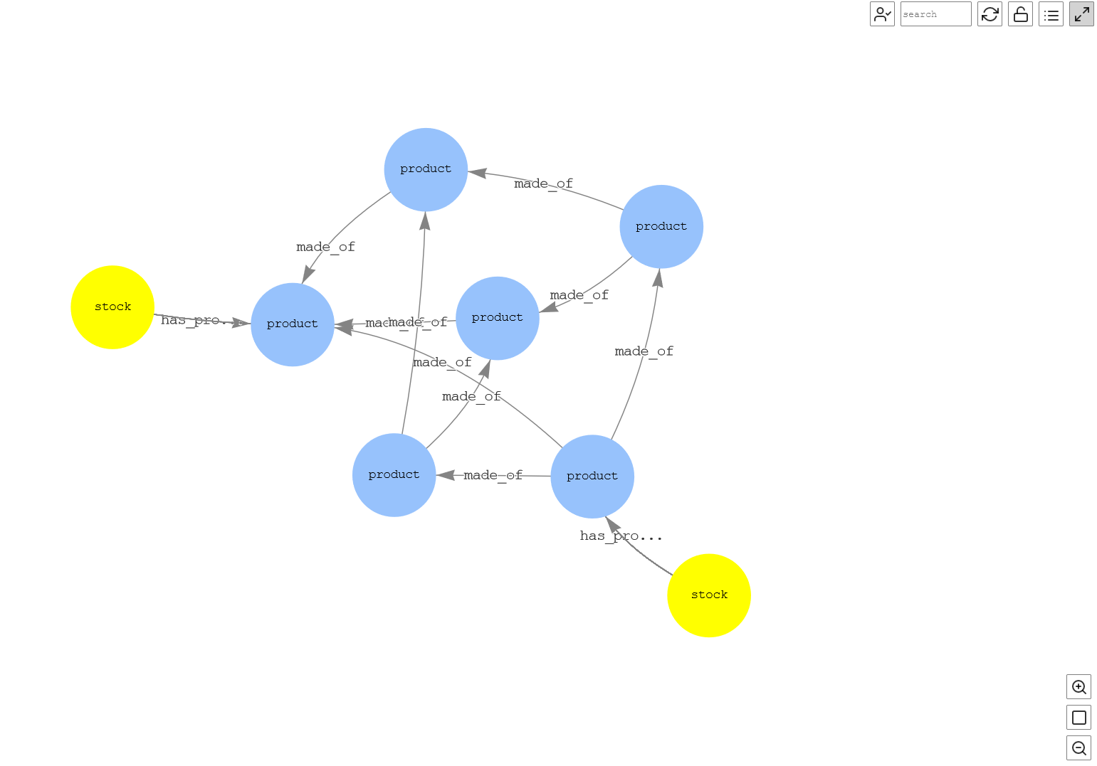
Figure-16: Stock for a product at a date

The final use case is to analyze the potential shortages in the supply chain, which is a very important part. The following query traverses the graph and finds out if a given product has any component that has a shortage that can affect the production of that particular product:

%%gremlin

// get potential shortages of components

g.V().
  has('name', 'Sedan Car').as('product').
  repeat(
    out('made_of').as('material').
    inE('has_product_in_stock').
    has('qty', lt(1)).as('stocklevel').
    outV().
    simplePath()).
    emit().
  select('material', 'stocklevel').by(elementMap('date', 'name', 'qty')).
  unfold()

The query returns the data showing that there will be a potential shortage of steel on August 2, 2022, at a certain warehouse.

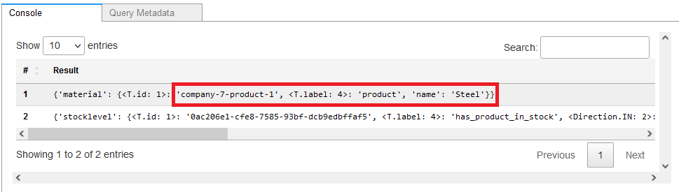
Figure-17a: Potential product for shortage

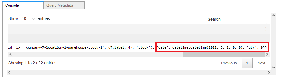
Figure-17b: Potential date shortage

Clean up

To avoid incurring future charges, delete the resources by deleting the CloudFormation stack you created for this post.

Conclusion

In this post, we showed how to analyze and visualize supply chain data through the Neptune graph database using the Gremlin query language. Today, innovative supply chain companies are looking to use graph analytics more and more to augment existing supply chain management systems, capture terabytes of data quickly, and gain unprecedented insights into their entire operations. Neptune graph databases help those companies innovate and take corrective actions whenever needed, for smooth functioning of their operations.

We invite you to try this post, post your comments and get more hands on through AWS graph notebook GitHub repo.

About the Authors

Dhiraj Thakur is a Solutions Architect with Amazon Web Services. He works with AWS customers and partners to provide guidance on enterprise cloud adoption, migration, and strategy. He is passionate about technology and enjoys building and experimenting in the analytics and AI/ML space.

Rajdip Chaudhuri is Senior Solutions Architect with Amazon Web Services specializing in data and analytics. He enjoys working with AWS customers and partners on data and analytics requirements. In his spare time, he enjoys soccer, movies.