AWS Physical AI Blog
Detect Objects in 3D LiDAR Point Clouds at Scale on AWS
This post is for machine learning and platform engineers who work with 3D Light Detection and Ranging (LiDAR) data and need to detect objects across large scans without hand-annotating every scene. You will learn how an open-source, event-driven pipeline on AWS ingests large point clouds, tiles them adaptively, runs 3D detection and segmentation, and returns reviewable results. It assumes familiarity with containers and Amazon Elastic Kubernetes Service, or Amazon EKS, but not with point cloud processing, and it stays at an architectural level while linking to the repository for implementation detail.
Why point cloud detection is hard to scale
LiDAR is now used on construction sites, in factories, on autonomous platforms, and in surveying rigs. Acquiring raw scans is straightforward. The hard part is turning a point cloud of tens or hundreds of millions of points into something usable, such as labeled objects, segmented structure, and measurements. That work is largely manual today, which makes it slow, expensive, and inconsistent between annotators, and it does not scale to the tens of gigabytes a single session can produce.
Teams often reach for image-based detection because it is easier to run, but projecting a 3D scene into 2D discards the geometry that makes LiDAR valuable. Point-cloud-native detection is memory and compute intensive, which is exactly the bursty workload the cloud handles well.
Teams also face a second problem, which is adapting models to their own domain and sensors. A model trained on indoor office environments will not perform well on construction sites without adaptation. This solution addresses both problems by pairing auto-scaling GPU and CPU inference on Amazon EKS with a built-in fine-tuning workflow, all from the same codebase.
Solution overview
The solution is an open, deployable pipeline that ingests large LiDAR scans in E57, LAS/LAZ, PLY, and KITTI .bin formats. It adaptively tiles the scene, runs 3D object detection and semantic segmentation, and returns structured results, including oriented bounding boxes, per-point class labels, and confidence scores. You review results in an interactive 3D web viewer or consume them as JSON.
The solution provides three core capabilities from a single codebase.
- Scalable inference on CPU or GPU, configurable per deployment
- Fine-tuning workflows that adapt detection and segmentation to your domain and sensors
- A local command-line interface, or CLI, for development and one-off scans with no cloud resources required
For teams and large workloads, it runs as a managed, event-driven service on Amazon EKS. The solution is container-based and portable, but this post focuses on Amazon EKS because it handles the bursty CPU and GPU workload mix most flexibly at production scale. Full setup, the CLI, the model zoo, and the output schema live in the repository.
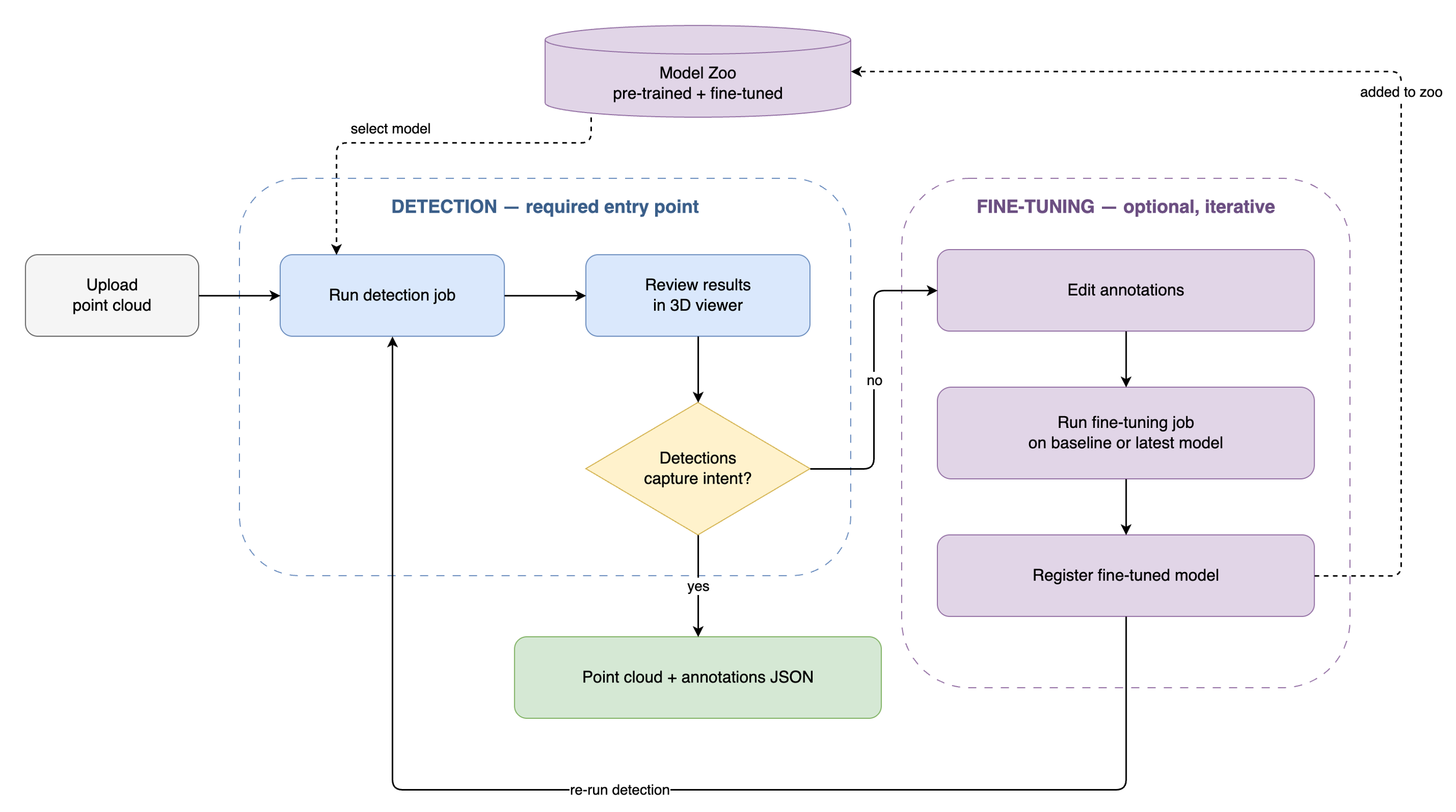
Figure 1. End-to-end workflow. A user uploads a scan, runs detection, and reviews results in the 3D viewer. An optional fine-tuning loop edits annotations, trains on a baseline or latest model, and returns the fine-tuned model to the model zoo.
Key capabilities
- Any scene size. Density-aware octree tiling handles scans from a single room to sites of 50 GB and larger within a configurable memory budget, 16 GB by default, then merges detections across tile boundaries.
- An interactive 3D viewer built for verifying results, with eye-dome-lighting depth shading, point coloring by height, RGB, intensity, or class, a semantic-segmentation overlay, and class and confidence filtering.
- A model zoo for real data. Indoor ScanNet, outdoor nuScenes, and KITTI models ship out of the box, plus the fine-tuning workflow below to close the domain gap for your sensor.
- FP16 precision support for faster GPU throughput on supported hardware.
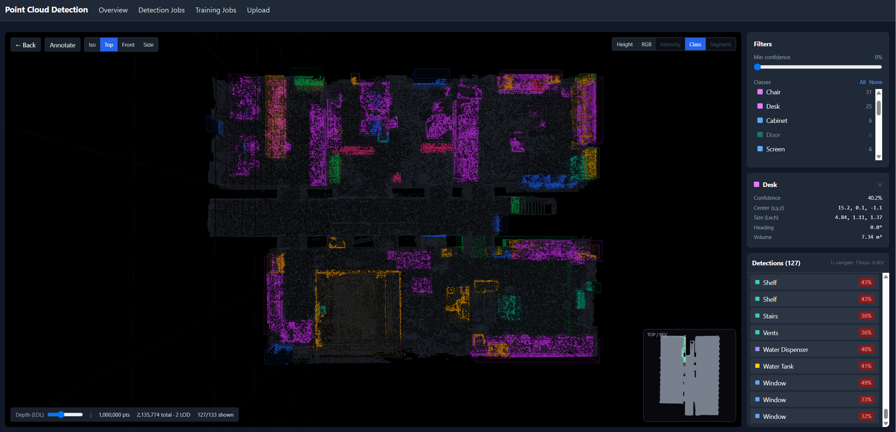
Figure 2. The interactive 3D viewer displaying LiDAR detections with class coloring, per-detection confidence, and class and confidence filtering.
Key design decisions
- Amazon EKS over AWS Fargate or Amazon SageMaker. The workload mixes CPU work such as I/O and tiling with bursty GPU inference, needs custom containers, and benefits from Kubernetes-native scaling.
- Event-driven with Amazon SQS, not a synchronous API. Detection can take minutes, so a queue decouples upload from processing, absorbs bursts, and provides retries and a dead-letter queue.
- CPU and GPU inference from the same codebase. The application auto-detects available hardware at runtime, GPU nodes give faster inference, CPU nodes save cost for latency-tolerant workloads, and GPU dependencies are optional.
- Scale-from-zero GPU nodes on Spot. The GPU node group scales up only when GPU work is queued and back to zero when idle, using Amazon EC2 Spot Instances to cut cost further.
- Least-privilege by default. Each workload gets its own IAM role through IAM Roles for Service Accounts (IRSA), so there are no shared node credentials, and all Amazon S3 buckets are encrypted at rest.
Architecture
The inference flow is event-driven.
- A user uploads a scan through the web UI, which streams it to Amazon Simple Storage Service, or Amazon S3, through a presigned multipart upload, so even very large files transfer reliably.
- A FastAPI service creates a job and enqueues a message on Amazon Simple Queue Service, or Amazon SQS.
- A worker fleet on Amazon EKS consumes the queue, reads the scan from Amazon S3, runs detection and segmentation, and writes results plus level-of-detail (LOD) viewer tiles back to Amazon S3.
- The UI polls job status and, when complete, streams the LOD tiles into a Three.js viewer for review.
- Failed jobs land on a dead-letter queue, and Amazon CloudWatch carries logs, metrics, and alarms throughout.
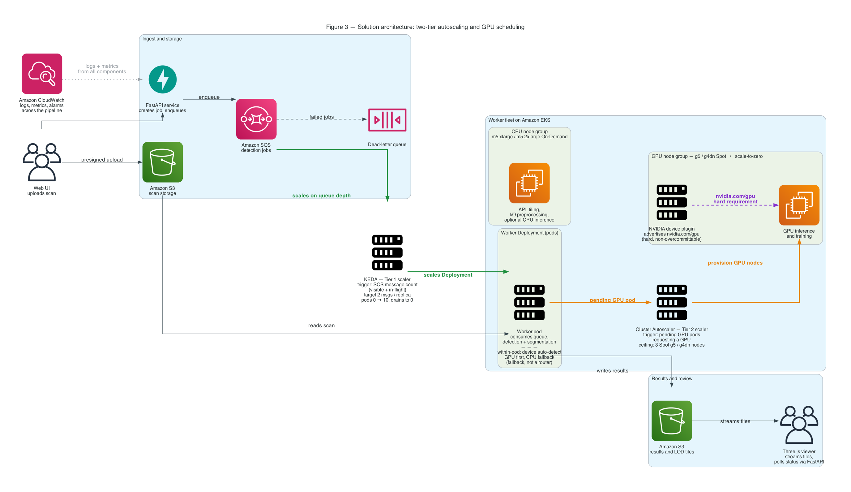
Figure 3. Solution architecture with two tiers of autoscaling. Tier 1 is KEDA scaling worker pods on Amazon SQS queue depth, and Tier 2 is the Cluster Autoscaler provisioning scale-to-zero GPU nodes for pending GPU pods, with the NVIDIA device plugin enforcing GPU scheduling. The event-driven data flow runs from scan upload through CPU or GPU detection to 3D review.
Compute configuration. The cluster provisions two node groups. CPU nodes running m5.xlarge or m5.2xlarge On-Demand instances handle the API, tiling, and I/O-heavy preprocessing, and can run CPU-based inference for teams that prefer lower cost over speed. GPU nodes running g5 or g4dn Spot instances scale from zero for GPU-accelerated inference and training, so you mostly pay for GPU while jobs run. If a Spot node is reclaimed mid-job, the Amazon SQS message returns to the queue and another worker retries automatically.
Turning queue depth into compute. Amazon EKS and Amazon SQS alone do not scale workers from a backlog, so the solution uses a two-tier control loop. Kubernetes Event-Driven Autoscaling (KEDA) scales worker pods from zero on Amazon SQS queue depth, counting in-flight as well as visible messages so a long-running job is never scaled away mid-flight. The Cluster Autoscaler then provisions GPU nodes for pending GPU pods, up to a fixed per-pool ceiling that caps cost regardless of backlog. Scaler targets, poll intervals, and cooldowns are in the repository.
How Kubernetes places GPU work. The key guarantee is that a GPU-intended job cannot silently run slowly on CPU. GPU pods request a GPU and tolerate a GPU-only node taint, GPU nodes carry the matching label and taint, and the NVIDIA device plugin advertises the GPU as a hard scheduling requirement. The worst case is a visibly pending pod waiting for a GPU node, which is observable and alertable. CPU versus GPU is a deployment-time choice today, not per-job routing, and the scheduling manifests are in the repository.
Cold start. The first job after scaling from zero is dominated by node provisioning and image pull, not inference.
| Phase | Observed time |
|---|---|
| GPU node launch, EC2 launch and cluster join | 2 to 4 min |
| Container image pull, 9 GB CUDA and PyTorch image, uncached | 4 to 5 min |
| Model load and checkpoint download | 15 to 20 sec |
| Total, first job on a freshly-scaled node | 6 to 9 min |
These are observed ranges from Kubernetes state transitions and worker logs, not controlled benchmarks, so treat them as directional. Once the node is warm and the image cached, latency is just inference time. Baking the checkpoint into the image removes the fetch from the cold path.
To configure the inference device, set inference.device to auto, cpu, or cuda:0 in the pipeline config file. On GPU deployments, pin cuda:0 so a misconfiguration fails loudly instead of silently running on CPU. See config.example.yaml in the repository for the full schema.
Adaptive tiling
Cutting a scene into tiles is the central technical contribution of the pipeline, and it comes down to three things, which are how you cut the scene, how much memory that costs, and how you merge the per-tile results. The pipeline handles all three with a density-aware, axis-qualified octree.
Axis-qualified means the octree splits only the axes still large enough to be worth splitting, so a cubic indoor room splits eight ways while a flat outdoor scene degrades cleanly to a quadtree instead of wasting tiles on empty air. Density-aware means each cut is placed at the point-count median rather than the geometric midpoint, so splits land in the sparse gaps between clusters instead of slicing through dense objects, and tiles end up with balanced point counts rather than balanced volume.
Tiles overlap by a configurable guard band so any object smaller than the band is seen whole by at least one tile. The memory budget is enforced two ways. The per-tile point cap is derived from the budget, and any scene whose modeled whole-load peak exceeds it is streamed rather than fully loaded, so peak memory stays bounded to a single tile even on scenes of 50 GB and larger. At the seams, a single 3D non-maximum-suppression pass removes duplicate boxes per class, and per-point labels in overlap zones keep the highest-confidence vote, so nothing is double-counted. Parameter defaults and the full streaming design are in the repository.
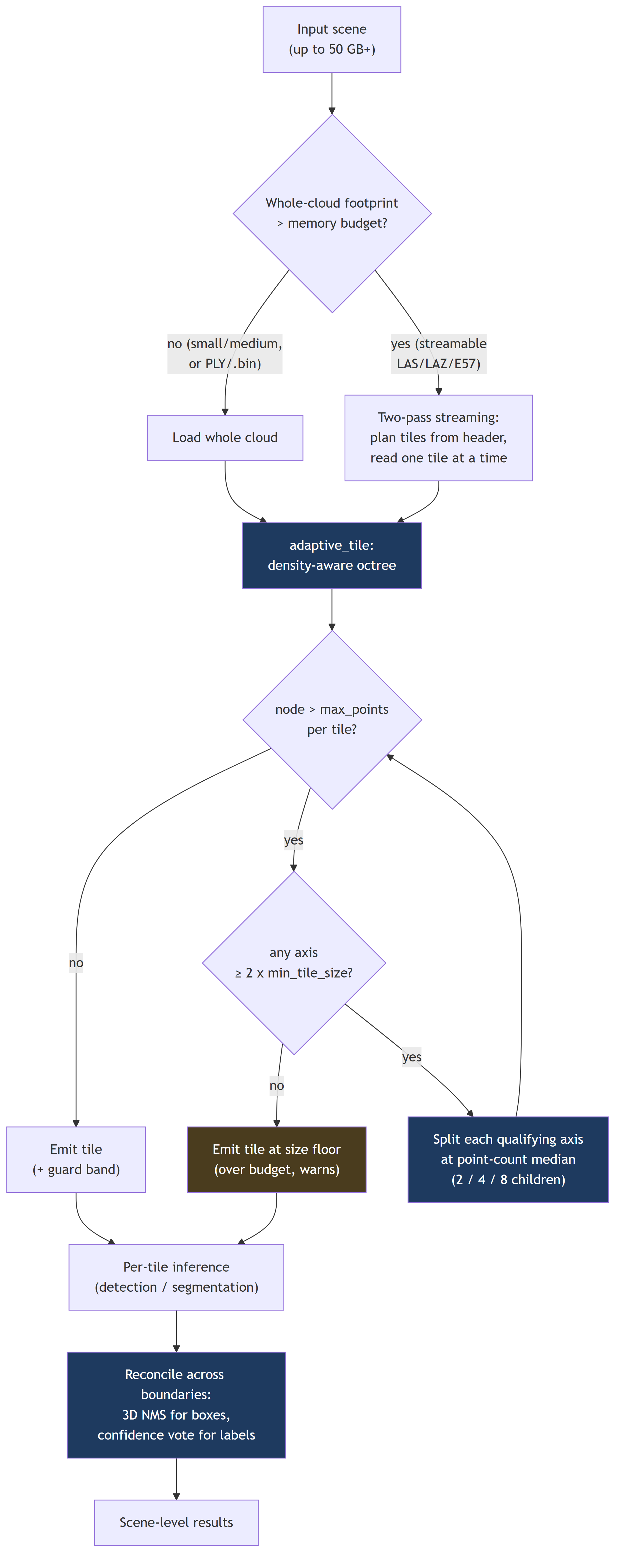
Figure 4. Adaptive tiling decision flow. The pipeline streams scenes that exceed the memory budget, subdivides a density-aware octree only on axes worth splitting, emits tiles with a guard band, and reconciles detections across boundaries with 3D non-maximum suppression.
Performance
The following results are throughput and memory measurements, not accuracy claims. The off-the-shelf models show a domain gap on industrial data, which is what the fine-tuning path addresses.
| Scan | Instance | Compute | Time | Peak memory |
|---|---|---|---|---|
| Leica factory scan, 25 GB, 1.46 B points, E57, 225 tiles | m5.2xlarge | CPU-only | 1 h 47 m | 9.5 GB |
| Streaming redesign scene, 300 M points | m5.2xlarge | CPU-only | 13 m 40 s | 2.56 GB |
| S3DIS conference room, 2.31 M points | g4dn.xlarge T4 | GPU, end-to-end service | about 9 sec | not recorded |
The 25 GB factory scan ran end-to-end under the 16 GB budget, with most tiles near 4 GB and the 9.5 GB peak from a single dense column. The store-once streaming redesign was decisive on the 300 M-point scene, cutting the run from over eight hours to under 14 minutes, roughly a 12x speedup with peak memory essentially flat. The 9-second conference-room result is end-to-end through the deployed service, from browser upload through Amazon SQS to a GPU worker and back to the viewer.
Fine-tuning for your domain
Out of the box, the model zoo includes pre-trained checkpoints for indoor scenes using ScanNet, outdoor environments using nuScenes, and autonomous driving using KITTI. Pre-trained models rarely reach production accuracy on a new sensor without adaptation, so the solution includes a complete fine-tuning workflow.
- Data preparation scripts for converting annotation formats such as nuScenes and SUSTechPoints, and for splitting train and validation sets
- Example fine-tuning configs for common scenarios such as doors, walls, and outdoor guardrails
- Custom class support, so you can define your own object classes or auto-detect them from annotations
- Local or Amazon EKS execution, to fine-tune locally during development, then submit a Kubernetes Job on GPU nodes for production datasets
- Evaluation tooling for measuring model accuracy before deployment
Training always runs on GPU. Once fine-tuning completes, the new weights are saved to the model registry in Amazon S3, referenced in the deployment config, and picked up on the next rollout.
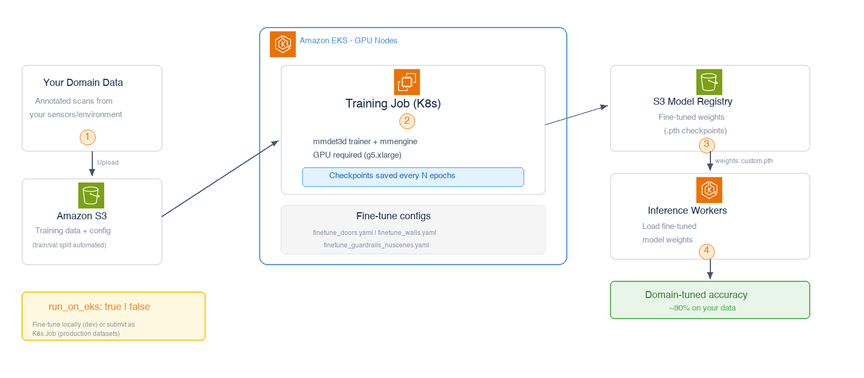
Figure 5. Fine-tuning workflow. Annotated domain data flows through a Kubernetes training job on GPU nodes, producing fine-tuned weights that inference workers pick up on the next rollout.
Bring your own model or detections
The detection backend separates architecture from weights, which opens three stable extension seams.
- Swap the weights, keep the pipeline. Point inference at your own checkpoint, as long as it is compatible with a shipped base architecture. Tiling, streaming, and post-processing are reused unchanged. A fine-tuned model with a new class list needs its class metadata wired in, not just the weights dropped in.
- Add a new architecture. Any model the detection framework supports is a small, bounded change, because everything downstream is architecture-agnostic.
- Bring your own detections. The viewer is driven by a documented results contract, so externally computed detections render with no code changes. This is also the path for importing your own ground-truth labels rather than drawing every box by hand.
Implementation detail for each seam is in the repository.
Getting started
Clone the repository and follow the quickstart in the README to run a local detection in minutes, with no cloud resources required. For the full managed deployment on Amazon EKS, the repository includes Terraform, Helm charts, and a step-by-step workshop that stands up the cluster, builds and pushes the images, and deploys the app. For fine-tuning, start with the model selection guide and one of the example configs.
- Repository, github.com/aws-samples/sample-point-cloud-object-detection-on-aws, with code, models, output schema, and architecture detail
- Workshop, in the workshop directory, to deploy end-to-end in roughly 2 to 4 hours
- Solution guidance, in docs/solution-guidance, for overview, deployment guide, cost, and FAQ
- Model selection guide, docs/MODEL_SELECTION_GUIDE.md, for choosing the right base model
- Annotation integration, docs/ANNOTATION_INTEGRATION.md, for connecting your labeling tools
Extending the solution
The solution is open-source and designed for extension. Common directions teams explore include the following.
- Fine-tuning with multi-modal inputs that combine image and point cloud data for higher accuracy
- Adding custom object classes beyond the pre-trained set
- Integrating the JSON output into downstream asset or analytics workflows
- Building per-job compute routing between CPU and GPU based on scan size or latency requirements
Conclusion
This post walked through an open-source, event-driven pipeline for detecting objects in 3D LiDAR point clouds at scale on AWS, combining density-aware tiling, a model zoo with indoor and outdoor pre-trained models, and a fine-tuning workflow that adapts detection to your domain. Running on Amazon EKS with configurable CPU and GPU node groups lets teams balance cost and performance, with GPU nodes scaling from zero on Spot to minimize idle spend. If you work with LiDAR and want to detect objects at scale without hand-annotating every scene, clone the repository, run a scan locally, open the results in the viewer, and send us feedback and contributions.