Using Spatial Data with Amazon Redshift

Today, Amazon Redshift announced support for a new native data type called GEOMETRY. This new type enables ingestion, storage, and queries against two-dimensional geographic data, together with the ability to apply spatial functions to that data. Geographic data (also known as georeferenced data) refers to data that has some association with a location relative to Earth. Coordinates, elevation, addresses, city names, zip (or postal) codes, administrative and socioeconomic boundaries are all examples of geographic data.

The GEOMETRY type enables us to easily work with coordinates such as latitude and longitude in our table columns, which can then be converted or combined with other types of geographic data using spatial functions. The type is abstract, meaning it cannot be directly instantiated, and polymorphic. The actual types supported for this data (and which will be used in table columns) are points, linestrings, polygons, multipoints, multilinestrings, multipolygons, and geometry collections. In addition to creating GEOMETRY-typed data columns in tables the new support also enables ingestion of geographic data from delimited text files using the existing COPY command. The data in the files is expected to be in hexadecimal Extended Well-Known Binary (EWKB) format which is a standard for representing geographic data.

To show the new type in action I imagined a scenario where I am working as a personal tour coordinator based in Berlin, Germany, and my client has supplied me with a list of attractions that they want to visit. My task is to locate accommodation for this client that is reasonably central to the set of attractions, and within a certain budget. Geographic data is ideal for solving this scenario. Firstly, the set of points representing the attractions combine to form one or more polygons which I can use to restrict my search for accommodation. In a single query I can then join the data representing those polygons with data representing a set of accommodations to arrive at the results. This spatial query is actually quite expensive in CPU terms yet Amazon Redshift is able to execute the query in less that one second.

Sample Scenario Data
To show my scenario in action I needed to first source various geographic data related to Berlin. Firstly I obtained the addresses, and latitude/longitude coordinates, of a variety of attractions in the city using several ‘top X things to see’ travel websites. For accommodation I used Airbnb data, licensed under the Creative Commons 1.0 Universal “Public Domain Dedication” from http://insideairbnb.com/get-the-data.html. I then added to this zip code data for the city, licensed under Creative Commons Attribution 3.0 Germany (CC BY 3.0 DE). The provider for this data is Amt für Statistik Berlin-Brandenburg.

Any good tour coordinator would of course have a web site or application with an interactive map so as to be able to show clients the locations of the accommodation that matched their criteria. In real life, I’m not a tour coordinator (outside of my family!) so for this post I’m going to focus solely on the back-end processes – the loading of the data, and the eventual query to satisfy our client’s request using the Amazon Redshift console.

Creating a Amazon Redshift Cluster
My first task is to load the various sample data sources into database tables in a Amazon Redshift cluster. To do this I go to the Amazon Redshift console dashboard and select Create cluster. This starts a wizard that walks me through the process of setting up a new cluster, starting with the type and number of nodes that I want to create.

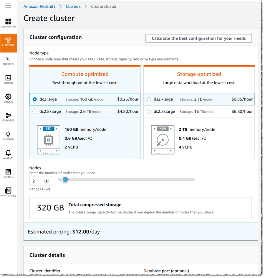
In Cluster details I fill out a name for my new cluster, set a password for the master user, and select an AWS Identity and Access Management (IAM) role that will give permission for Amazon Redshift to access one of my buckets in Amazon Simple Storage Service (Amazon S3) in read-only mode when I come to load my sample data later. The new cluster will be created in my default Amazon Virtual Private Cloud (Amazon VPC) for the region, and I also opted to use the defaults for node types and number of nodes. You can read more about available options for creating clusters in the Management Guide. Finally I click Create cluster to start the process, which will take just a few minutes.

Loading the Sample Data
With the cluster ready to use I can load the sample data into my database, so I head to the Query editor and using the pop-up, connect to my default database for the cluster.

My sample data will be sourced from delimited text files that I’ve uploaded as private objects to an Amazon S3 bucket and loaded into three tables. The first, accommodations, will hold the Airbnb data. The second, zipcodes, will hold the zip or postal codes for the city. The final table, attractions, will hold the coordinates of the city attractions that my client can choose from. To create and load the accommodations data I paste the following statements into tabs in the query editor, one at a time, and run them. Note that schemas in databases have access control semantics and the public prefix shown on the table names below simply means I am referencing the public schema, accessible to all users, for the database in use.

To create the accommodations table I use:

CREATE TABLE public.accommodations (
  id INTEGER PRIMARY KEY,
  shape GEOMETRY,
  name VARCHAR(100),
  host_name VARCHAR(100),
  neighbourhood_group VARCHAR(100),
  neighbourhood VARCHAR(100),
  room_type VARCHAR(100),
  price SMALLINT,
  minimum_nights SMALLINT,
  number_of_reviews SMALLINT,
  last_review DATE,
  reviews_per_month NUMERIC(8,2),
  calculated_host_listings_count SMALLINT,
  availability_365 SMALLINT
);

To load the data from Amazon S3:

COPY public.accommodations
FROM 's3://my-bucket-name/redshift-gis/accommodations.csv'
DELIMITER ';'
IGNOREHEADER 1
CREDENTIALS 'aws_iam_role=arn:aws:iam::123456789012:role/RedshiftDemoRole';

Next, I repeat the process for the zipcodes table.

CREATE TABLE public.zipcode (
  ogc_field INTEGER,
  wkb_geometry GEOMETRY,
  gml_id VARCHAR,
  spatial_name VARCHAR,
  spatial_alias VARCHAR,
  spatial_type VARCHAR
);

COPY public.zipcode
FROM 's3://my-bucket-name/redshift-gis/zipcode.csv'
DELIMITER ';'
IGNOREHEADER 1
IAM_ROLE 'arn:aws:iam::123456789012:role/RedshiftDemoRole';

And finally I create the attractions table and load data into it.

CREATE TABLE public.berlin_attractions (
  name VARCHAR,
  address VARCHAR,
  lat DOUBLE PRECISION,
  lon DOUBLE PRECISION,
  gps_lat VARCHAR,
  gps_lon VARCHAR
);

COPY public.berlin_attractions
FROM 's3://my-bucket-name/redshift-gis/berlin-attraction-coordinates.txt'
DELIMITER '|'
IGNOREHEADER 1
IAM_ROLE 'arn:aws:iam::123456789012:role/RedshiftDemoRole';

Finding Somewhere to Stay!
With the data loaded, I can now put on my travel coordinator hat and select some properties for my client to consider for their stay in Berlin! Remember, in the real world this would likely be surfaced from a web or other application for the client. I’m simply going to make use of the query editor again.

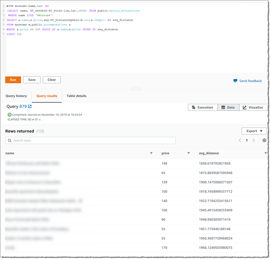
My client has decided they want a trip to focus on the city museums and they have a budget of 200 EUR per night for accommodation. Opening a new tab in the editor, I paste in and run the following query.

WITH museums(name,loc) AS
(SELECT name, ST_SetSRID(ST_Point(lon,lat),4326) FROM public.berlin_attractions
WHERE name LIKE '%Museum%')
SELECT a.name,a.price,avg(ST_DistanceSphere(m.loc,a.shape)) AS avg_distance
FROM museums m,public.accommodations a
WHERE a.price <= 200 GROUP BY a.name,a.price ORDER BY avg_distance
LIMIT 10;

The query finds the accommodation(s) that are “best located” to visit all the museums, and whose price is within the client’s budget. Here “best located” is defined as having the smallest average distance from all the selected museums. In the query you can see some of the available spatial functions, ST_SetSRID and ST_Point, operating on the latitude and longitude GEOMETRY columns for the attractions, and ST_DistanceSphere to determine distance.

This yields the following results.

Wrap a web or native application front-end around this and we have a new geographic data-based application that we can use to delight clients who have an idea of what they want to see in the city and also want convenient and in-budget accommodation best placed to enable that!

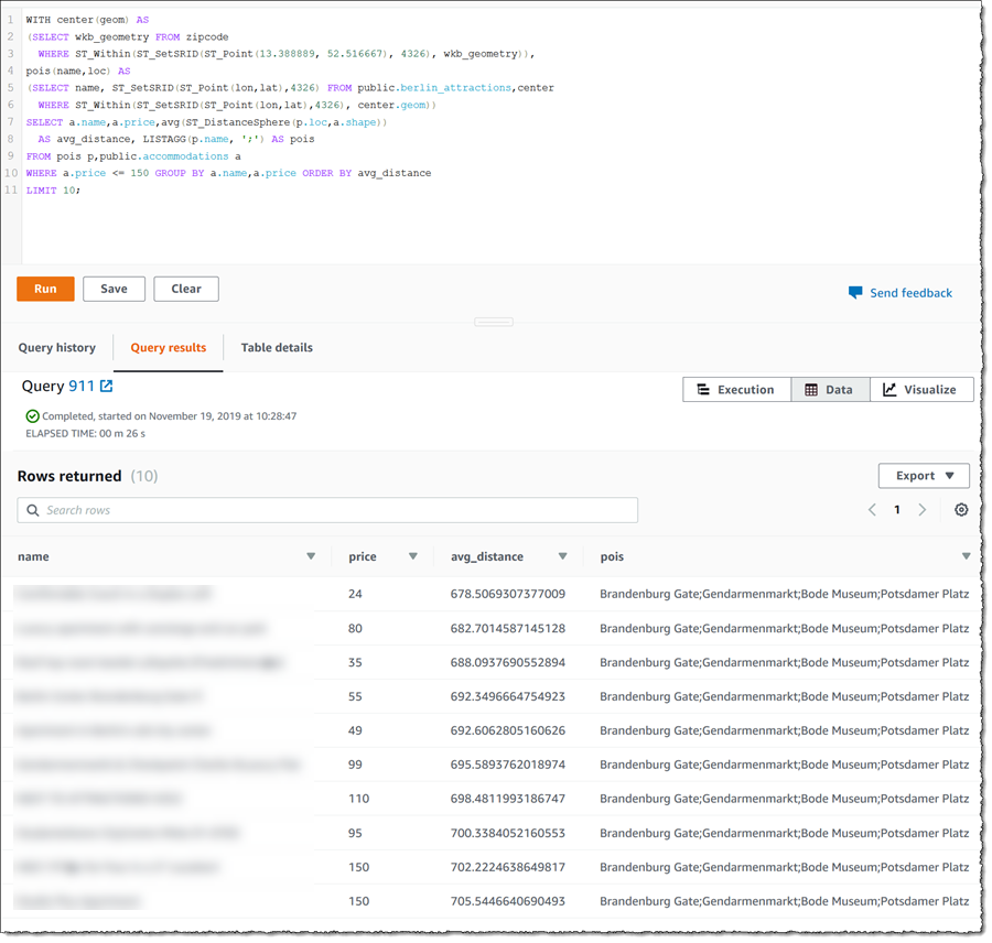
Let’s also consider another scenario. Imagine I have a client who wants to stay in the center of Berlin but isn’t sure what attractions or accommodations are present in the central district, and has a budget of 150 EUR per night. How can we answer that question? First we need the coordinates of what we might consider to be the center of Berlin – latitude 52.516667, longitude 13.388889. Using the zipcode table we can convert this coordinate location to a polygon enclosing that region of the city. Our query must then get all attractions within that polygon, plus all accommodations (within budget), ordered by average distance from the attractions. Here’s the query:

WITH center(geom) AS
(SELECT wkb_geometry FROM zipcode
  WHERE ST_Within(ST_SetSRID(ST_Point(13.388889, 52.516667), 4326), wkb_geometry)),
pois(name,loc) AS
(SELECT name, ST_SetSRID(ST_Point(lon,lat),4326) FROM public.berlin_attractions,center
  WHERE ST_Within(ST_SetSRID(ST_Point(lon,lat),4326), center.geom))
SELECT a.name,a.price,avg(ST_DistanceSphere(p.loc,a.shape))
  AS avg_distance, LISTAGG(p.name, ';') as pois
FROM pois p,public.accommodations a
WHERE a.price <= 150 GROUP BY a.name,a.price ORDER BY avg_distance
LIMIT 10;

When I run this in the query editor, I get the following results. You can see the list of attractions in the area represented by the zipcode in the pois column.

So there we have some scenarios for making use of geographic data in Amazon Redshift using the new GEOMETRY type and associated spatial functions, and I’m sure there are many more! The new type and functions are available now in all AWS Regions to all customers at no additional cost.