Building a scalable, transactional data lake using dbt, Amazon EMR, and Apache Iceberg

Growing data volume, variety, and velocity has made it crucial for businesses to implement architectures that efficiently manage and analyze data, while maintaining data integrity and consistency. In this post, we show you a solution that combines Apache Iceberg, Data Build Tool (dbt), and Amazon EMR to create a scalable, ACID-compliant transactional data lake. You can use this data lake to process transactions and analyze data simultaneously while maintaining data accuracy and real-time insights for better decision-making.

Challenges, business imperatives, and technical advantages

Traditional data lakes have long struggled with fundamental limitations. For example, the lack of ACID compliance, data inconsistencies from concurrent writes, complex schema evolution, and the absence of time travel, rollback, and versioning capabilities. These shortcomings directly conflict with growing business demands for concurrent read/write support, robust data versioning and auditing, schema flexibility, and transactional capability within data lake environments. To address these gaps, modern solutions use ACID transactions at scale, optimized storage formats through Apache Iceberg, version control for data on Amazon Simple Storage Service (Amazon S3), and cost-effective, streamlined maintenance—delivering a reliable, enterprise-grade data lake architecture that meets both operational and analytical needs.

Solution overview

The solution is built around four tightly integrated layers that work together to deliver a scalable, transactional data lake.

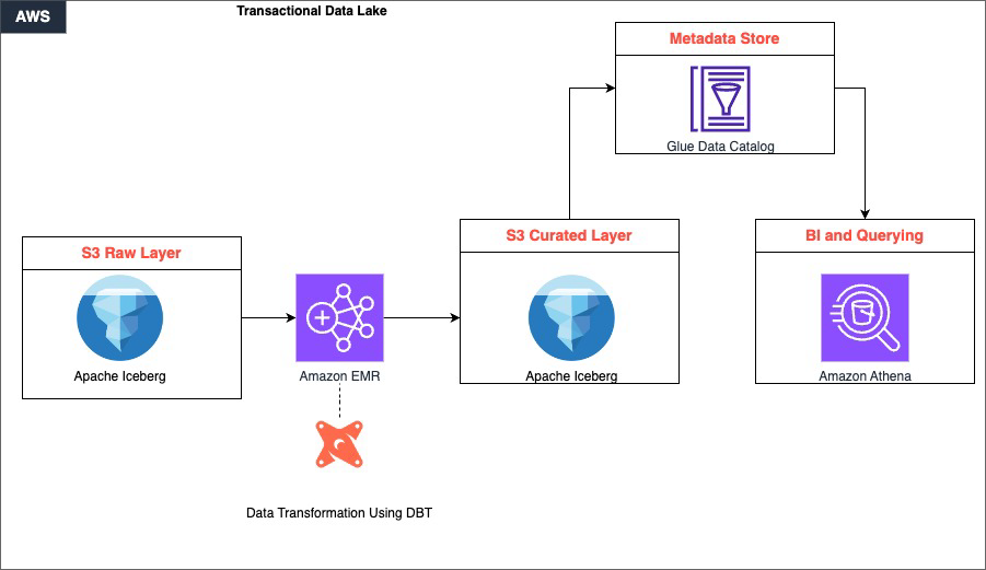
Raw data is ingested and stored in Amazon S3, which serves as the foundational storage layer. This layer supports multiple data formats and enables efficient data partitioning through Apache Iceberg’s table format. This ensures that data is organized and accessible from the moment it lands. Then, Amazon EMR takes over as the distributed computing engine, using Apache Spark to process large-scale datasets in parallel, handling the heavy lifting of reading, transforming, and writing data across the lake.

Sitting within the processing layer, dbt drives the transformation logic. It applies SQL-based, version-controlled transformations that convert raw, unstructured data in the S3 raw layer into clean, curated datasets stored back in S3. This maintains ACID compliance and schema consistency throughout.

Finally, the curated data is available for consumption through Amazon Athena, which provides a serverless, one-time querying capability directly on S3. With this, analysts and business users can run interactive SQL queries without managing any infrastructure. Together, these components form a continuous pipeline: data flows from ingestion through distributed processing and structured transformation, ultimately surfacing as reliable, query-ready insights.

Amazon EMR is a cloud-based big data service that streamlines the deployment and management of open source frameworks like Apache Spark, Hive, and Trino. It provides a managed Apache Hadoop environment that organizations can use to process and analyze vast amounts of data efficiently.

Data Build Tool is an open source tool that data teams can use to transform and model data using SQL. It promotes best practices for data modeling, testing, and documentation, streamlining maintenance and collaboration on data pipelines.

Apache Iceberg is an open table format designed for large-scale analytics on data lakes. It supports features like transactions, time travel, and data partitioning, which are essential for building reliable and performant data lakes. By using Iceberg, organizations can maintain data integrity and enable efficient querying and processing of data.

When combined, these three technologies provide a powerful solution for building transactional data lakes. Amazon EMR provides the scalable and managed infrastructure for running big data workloads, dbt enables efficient data modeling and transformation, and Apache Iceberg provides data consistency and reliability within the data lake.

Prerequisites

Before proceeding with the solution walkthrough, make sure that the following are in place:

• AWS Account – An active AWS account with sufficient permissions to create and manage EMR clusters, S3 buckets, Athena workgroups, and AWS Glue Data Catalog resources
• IAM Roles – The following IAM roles must exist and have appropriate permissions:
  • EMR_DefaultRole – Service role for Amazon EMR
  • EMR_EC2_DefaultRole – Amazon Elastic Compute Cloud (Amazon EC2) instance profile for EMR nodes
• AWS Command Line Interface (AWS CLI) – Installed and configured with credentials for your target AWS account and AWS Region (refer to Step 1.1 for setup instructions)
• Python 3.8+ – Installed on your local machine or workspace for setting up the dbt virtual environment
• Pip – Python package manager available for installing dbt and its dependencies
• Git – Installed on the EMR primary node or local environment for version control and dbt package management
• Amazon Athena – Athena query editor access with a configured S3 output location for query results
• AWS Glue Data Catalog – Enabled as the metastore for Amazon EMR and Athena (no additional setup required if using the default AWS Glue integration)
• S3 Bucket Naming – Prepare a unique identifier to suffix S3 bucket names, ensuring global uniqueness across all three buckets created in Step 1.3
• Network Access – Make sure that your local machine can reach the Amazon EMR primary node’s DNS over port 10001 (Thrift/HiveServer2) for dbt connectivity; configure security groups accordingly

Solution walkthrough

Step 1: Environment setup

1. Install the AWS CLI on your workspace by following the instructions in Installing or updating the latest version of the AWS CLI. To configure AWS CLI interaction with AWS, refer to Quick setup.
2. Create EMR cluster.

   Create the following JSON file with the following contents emr-config.json:

   [
     {
       "Classification": "iceberg-defaults",
       "Properties": {
         "iceberg.enabled": "true"
       }
     },
     {
       "Classification": "spark-hive-site",
       "Properties": {
         "hive.metastore.client.factory.class": "com.amazonaws.glue.catalog.metastore.AWSGlueDataCatalogHiveClientFactory"
       }
     }
   ]

   Run the following command on your AWS CLI, updating the preferred AWS Region:

   aws emr create-cluster \
   --name "Iceberg-DBT-Cluster" \
   --release-label emr-7.7.0 \
   --applications Name=Spark Name=Hive Name=Livy \
   --ec2-attributes InstanceProfile=EMR_EC2_DefaultRole \
   --instance-type c3.4xlarge \
   --instance-count 1 \
   --service-role EMR_DefaultRole \
   --configurations file://emr-config.json \
   --region [region]

3. Set up S3 buckets.
   Create the following S3 bucket using the AWS CLI after updating the bucket name.

   aws s3 mb s3://amzn-s3-demo-transactional-datalake-raw-[unique-identifier]
   aws s3 mb s3://amzn-s3-demo-transactional-datalake-curated-[unique-identifier]
   aws s3 mb s3://amzn-s3-demo-transactional-datalake-analytics-[unique-identifier]
   

Step 2. Raw layer implementation

The raw layer serves as the foundation of our data lake, ingesting and storing data in its original form. This layer is important for maintaining data lineage and enabling reprocessing if needed. We use Apache Iceberg tables to store our raw data, which provides benefits such as ACID transactions, schema evolution, and time travel capabilities.

In this step, we create a dedicated database for our raw data and set up tables for customers, products, and sales using Amazon Athena. These tables are configured to use the Iceberg table format and are compressed using the ZSTD algorithm to optimize storage. The LOCATION property specifies where the data will be stored in Amazon S3 so that data is organized and accessible.

After creating the tables, we insert sample data to simulate real-world scenarios. We use this data throughout the rest of the implementation to demonstrate the capabilities of our data lake architecture.

Update the respective bucket name in each create table bucket name from the previous step:

1. Create database and tables

   -- Create Raw Database
   CREATE SCHEMA raw_sales_analytics_data_layer;
   
   -- Create Customers Table
   CREATE TABLE raw_sales_analytics_data_layer.customers (
       CustomerID string,
       CustomerName string,
       Region string,
       inserted_timestamp timestamp
   )
   LOCATION 's3://[bucket_name]/raw_sales_analytics_data_layer/customers'
   TBLPROPERTIES (
       'table_type'='iceberg', 
       'write_compression'='zstd'
   );
   
   -- Create Products Table
   CREATE TABLE raw_sales_analytics_data_layer.products (
       productid string,
       productname string,
       category string,
       supplier string,
       inserted_timestamp timestamp
   )
   LOCATION 's3://[bucket_name]/raw_sales_analytics_data_layer/products'
   TBLPROPERTIES (
       'table_type'='iceberg', 
       'write_compression'='zstd'
   );

2. Insert sample data

   -- Insert Customers
   INSERT INTO raw_sales_analytics_data_layer.customers
   VALUES 
       ('201', Jane Doe', 'Central', current_timestamp),
       ('202', Arnav Desai, 'North', current_timestamp),
       ('203', Kwaku Mensah, 'West', current_timestamp);
   
   -- Insert Products
   INSERT INTO raw_sales_analytics_data_layer.products
   VALUES
       ('1', 'Laptop', 'Electronics', 'AnyAuthority', current_timestamp),
       ('2', 'Smartphone', 'Electronics', 'AnyCompany', current_timestamp);
   
   -- Insert Sales
   INSERT INTO raw_sales_analytics_data_layer.sales
   VALUES
       ('ORD001', '1', '201', '2025-04-01', 1299.99, current_timestamp),
       ('ORD002', '2', '202', '2025-04-02', 899.99, current_timestamp);

Step 3: dbt setup and configuration

Setting up dbt involves installing the necessary packages, configuring the connection to the data warehouse (in this case, Amazon EMR), and setting up the project structure.

We start by creating a Python virtual environment to isolate our dbt installation. Then, we install dbt-core and the Spark adapter, which allows dbt to connect to the EMR cluster. The profiles.yml file is configured to connect to the EMR cluster using the Thrift protocol, while the dbt_project.yml file defines the overall structure of the dbt project, including model materialization strategies and file formats.

1. Install prerequisites

   # Create Python virtual environment
   python -m venv dbt-env
   source dbt-env/bin/activate
   
   # Install required packages
   pip install dbt-core dbt-spark[PyHive]
   
   # Install git
   yum install git

2. Configure dbt profiles

   # ~/.dbt/profiles.yml
   sales_analytics:
     target: dev
     outputs:
       dev:
         type: spark
         method: thrift
         host: your-emr-master-dns
         port: 10001
         schema: curated_sales_analytics_data_layer
         threads: 4

3. Project configuration

   # dbt_project.yml
   name: 'sales_analytics'
   version: '1.0.0'
   config-version: 2
   
   profile: 'sales_analytics'
   
   model-paths: ["models"]
   analysis-paths: ["analyses"]
   test-paths: ["tests"]
   seed-paths: ["seeds"]
   macro-paths: ["macros"]
   
   target-path: "target"
   clean-targets:
       - "target"
       - "dbt_packages"
   
   models:
     sales_analytics:
       dim:
         +materialized: table
         +file_format: iceberg
       ads:
         +materialized: table
         +file_format: iceberg

Step 4: dbt models implementation

In this step, we implement dbt models, which define the transformations that we will apply to raw data. We start by configuring data sources in the sources.yml file, which allows dbt to reference raw tables easily.

We then create dimension models for customers and products, and a fact model for sales.

These models use incremental materialization strategies to efficiently update data over time. The incremental strategy processes only new or updated records, significantly reducing the time and resources required for each run.

1. Source configuration

   # models/sources.yml
   version: 2
   sources:
     - name: raw_sales
       database: raw_sales_analytics_data_layer
       schema: raw_sales_analytics_data_layer
       tables:
         - name: customers
           columns:
             - name: CustomerID
               tests:
                 - unique
                 - not_null
         - name: products
         - name: sales

2. Dimension models

   -- models/dim/dim_customers.sql
   {{ config(
       materialized='incremental',
       unique_key='customerid',
       incremental_strategy='merge'
   ) }}
   
   WITH source_data AS (
       SELECT 
           customerid,
           customername,
           region,
           inserted_timestamp,
           ROW_NUMBER() OVER (
               PARTITION BY customerid 
               ORDER BY inserted_timestamp DESC
           ) as row_number
       FROM {{ source('raw_sales_analytics_data_layer', 'customers') }}
       {% if is_incremental() %}
       WHERE inserted_timestamp > (SELECT MAX(inserted_timestamp) FROM {{ this }})
       {% endif %}
   )
   
   SELECT 
       customerid,
       customername,
       region,
       inserted_timestamp
   FROM source_data
   WHERE row_number = 1

3. Product models

   -- models/dim/dim_products.sql
   {{ config(
       materialized='incremental',
       unique_key='productid',
       incremental_strategy='merge'
   ) }}
   
   WITH source_data AS (
       SELECT
           productid,
           productname,
           category,
           supplier,
           inserted_timestamp,
           ROW_NUMBER() OVER (
               PARTITION BY productid
               ORDER BY inserted_timestamp DESC
           ) as row_number
       FROM {{ source('raw_sales_analytics_data_layer', 'products') }}
       {% if is_incremental() %}
       WHERE inserted_timestamp > (SELECT MAX(inserted_timestamp) FROM {{ this }})
       {% endif %}
   )
   
   SELECT
       s.productid,
       s.productname,
       s.category,
       s.supplier,
       s.inserted_timestamp
   FROM source_data s
   WHERE s.row_number = 1
   {% if is_incremental() %}
       AND NOT EXISTS (
           SELECT 1
           FROM {{ this }} t
           WHERE t.productid = s.productid
           AND t.inserted_timestamp >= s.inserted_timestamp
       )
   {% endif %}

4. Fact models

   -- models/dim/fact_sales.sql
   {{ config(
       materialized='incremental',
       unique_key='orderid',
       incremental_strategy='merge'
   ) }}
   
   WITH source_data AS (
       SELECT
           orderid,
           productid,
           customerid,
           date,
           salesamount,
           inserted_timestamp,
           ROW_NUMBER() OVER (
               PARTITION BY orderid
               ORDER BY inserted_timestamp DESC
           ) as row_number
       FROM {{ source('raw_sales_analytics_data_layer', 'sales') }}
       {% if is_incremental() %}
       WHERE orderid NOT IN (SELECT orderid FROM {{ this }})  -- Changed condition
       {% endif %}
   )
   
   SELECT
       s.orderid,
       s.productid,
       s.customerid,
       s.date,
       s.salesamount,
       s.inserted_timestamp
   FROM source_data s
   WHERE s.row_number = 1

Step 5: Analytics layer

The analytics layer builds upon dimension and fact models to create more complex analyzes. In this step, we create a daily sales analysis model that combines data from fact_sales, dim_customers, and dim_products models.

We also implement a customer insights model that analyzes purchase patterns across different Regions and product categories.

These analytics models demonstrate how we can use our transformed data to generate valuable business insights. By materializing these models as Iceberg tables, we make sure that they benefit from the same ACID transactions and time travel capabilities as our raw and transformed data.

1. Daily sales analysis

   The analytics layer introduces a fact_sales_analysis model that consolidates transactional sales data with customer and product dimensions to enable business-ready reporting. Built as an incremental model with a merge strategy, it efficiently processes data by deduplicating records using the latest inserted timestamp per order, enabling reliable downstream consumption without full table refreshes.

   -- models/ads/fact_sales_analysis.sql
   {{ config(
       materialized='incremental',
       unique_key='orderid',
       incremental_strategy='merge'
   ) }}
   
   WITH source_data AS (
       SELECT
           s.orderid,
           s.date,
           s.salesamount,
           c.customername,
           c.region,
           p.productname,
           p.category,
           p.supplier,
           s.inserted_timestamp,
           ROW_NUMBER() OVER (
               PARTITION BY s.orderid
               ORDER BY s.inserted_timestamp DESC
           ) as row_number
       FROM {{ ref('fact_sales') }} s
       JOIN {{ ref('dim_customers') }} c ON s.customerid = c.customerid
       JOIN {{ ref('dim_products') }} p ON s.productid = p.productid
       {% if is_incremental() %}
       WHERE s.orderid NOT IN (SELECT orderid FROM {{ this }})
       {% endif %}
   )
   
   SELECT
       s.orderid,
           s.date,
           s.salesamount,
           s.customername,
           s.region,
           s.productname,
           s.category,
           s.supplier,
           s.inserted_timestamp
   FROM source_data s
   WHERE s.row_number = 1

2. Customer insights

   The customer_purchase_patterns model aggregates sales activity across customer Regions and product categories to surface revenue trends and buying behavior. Materialized as an Iceberg table in the analytics schema, it provides a performant and scalable foundation for customer segmentation, Regional performance analysis, and category-level revenue attribution.

   -- models/analytics/customer_purchase_patterns.sql
   {{
       config(
           materialized='table',
           file_format='iceberg',
           schema='analytics'
       )
   }}
   
   SELECT
       dc.Region,
       dp.category,
       COUNT(DISTINCT fs.orderid) as total_orders,
       COUNT(DISTINCT dc.customerid) as unique_customers,
       SUM(fs.salesamount) as total_revenue,
       SUM(fs.salesamount) / COUNT(DISTINCT dc.customerid) as revenue_per_customer
   FROM {{ ref('fact_sales') }} fs
   JOIN {{ ref('dim_customers') }} dc ON fs.customerid = dc.customerid
   JOIN {{ ref('dim_products') }} dp ON fs.productid = dp.productid
   GROUP BY dc.Region, dp.category

Step 6: Transactional operations and time travel with Apache Iceberg

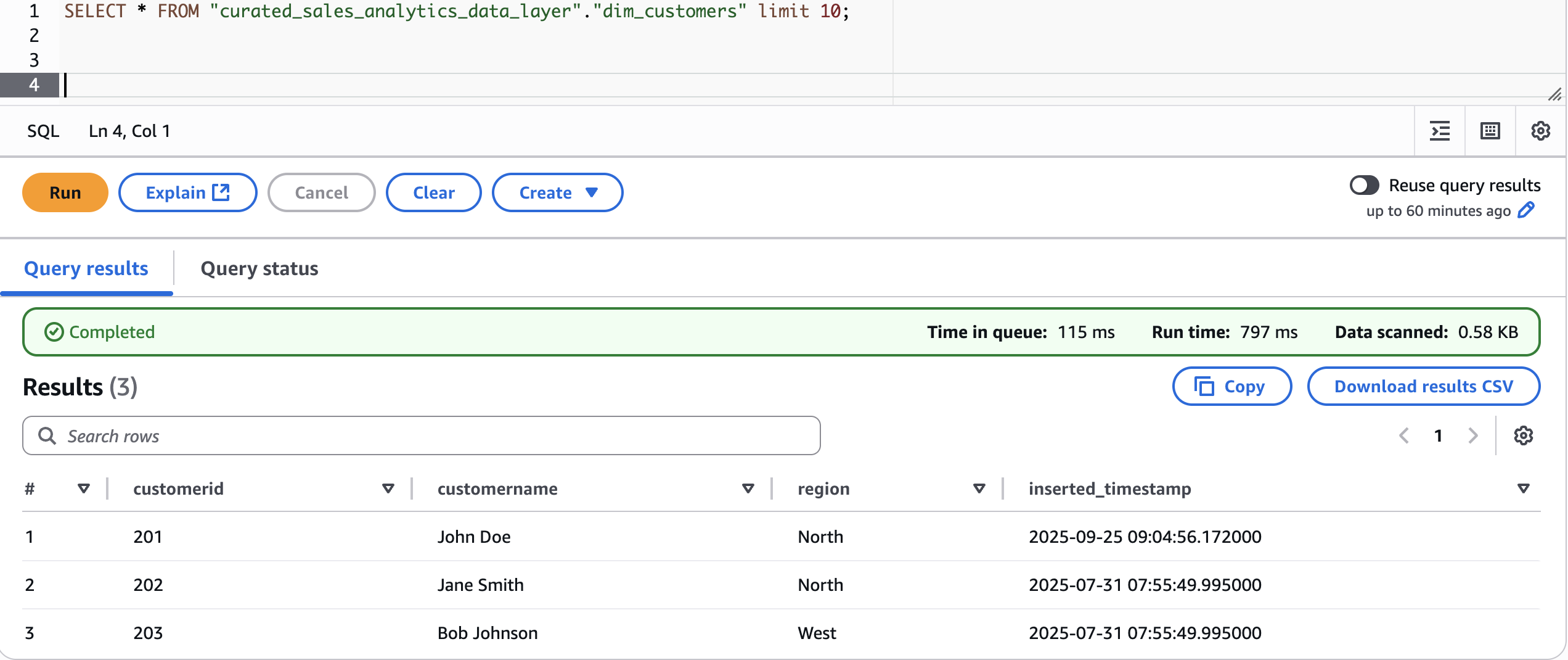
This section demonstrates how to use Apache Iceberg’s time travel capabilities and transactional operations using actual snapshot data from our dim_customers table. We walk through querying data at different points in time and comparing changes between snapshots.

1. Transactional capabilities

   Let’s first look at current data:

   

   Now, modify the raw layer data for customerid 201 and change the Region to East

   

   Run the dbt model for dim_customers to sync the changes

   

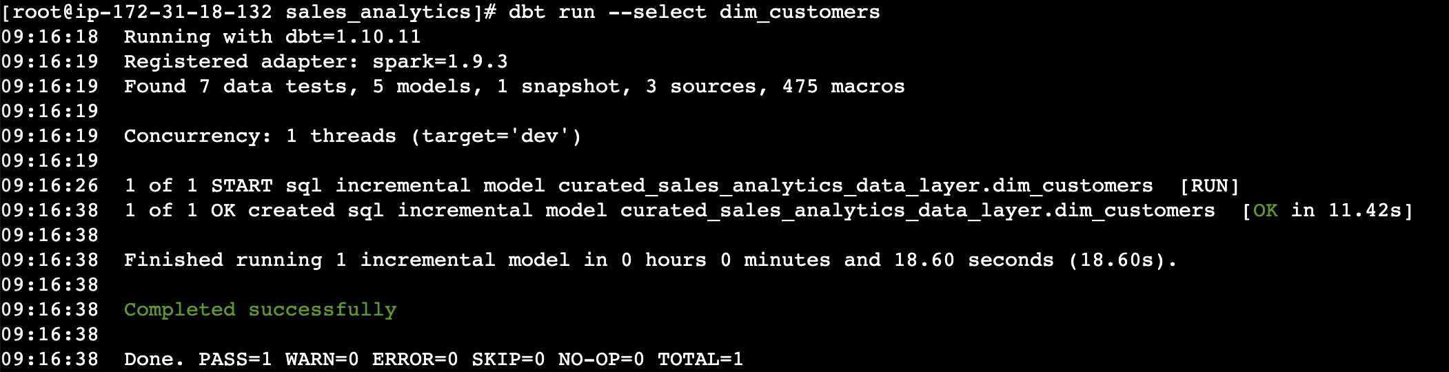
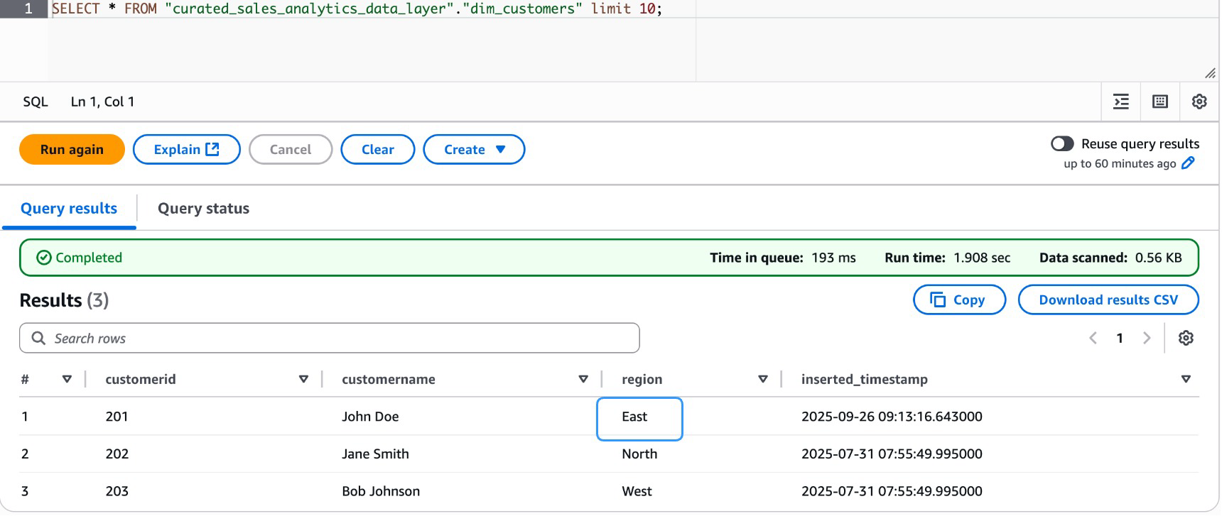
   Validate the data in curated layer for dim_customers dimension table

   

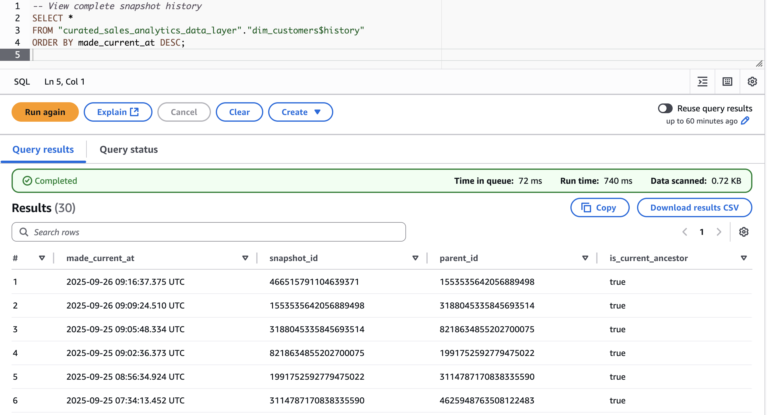
2. Time-travel capabilities

   First, let’s fetch snapshots for customers dimension table in curated layer

   

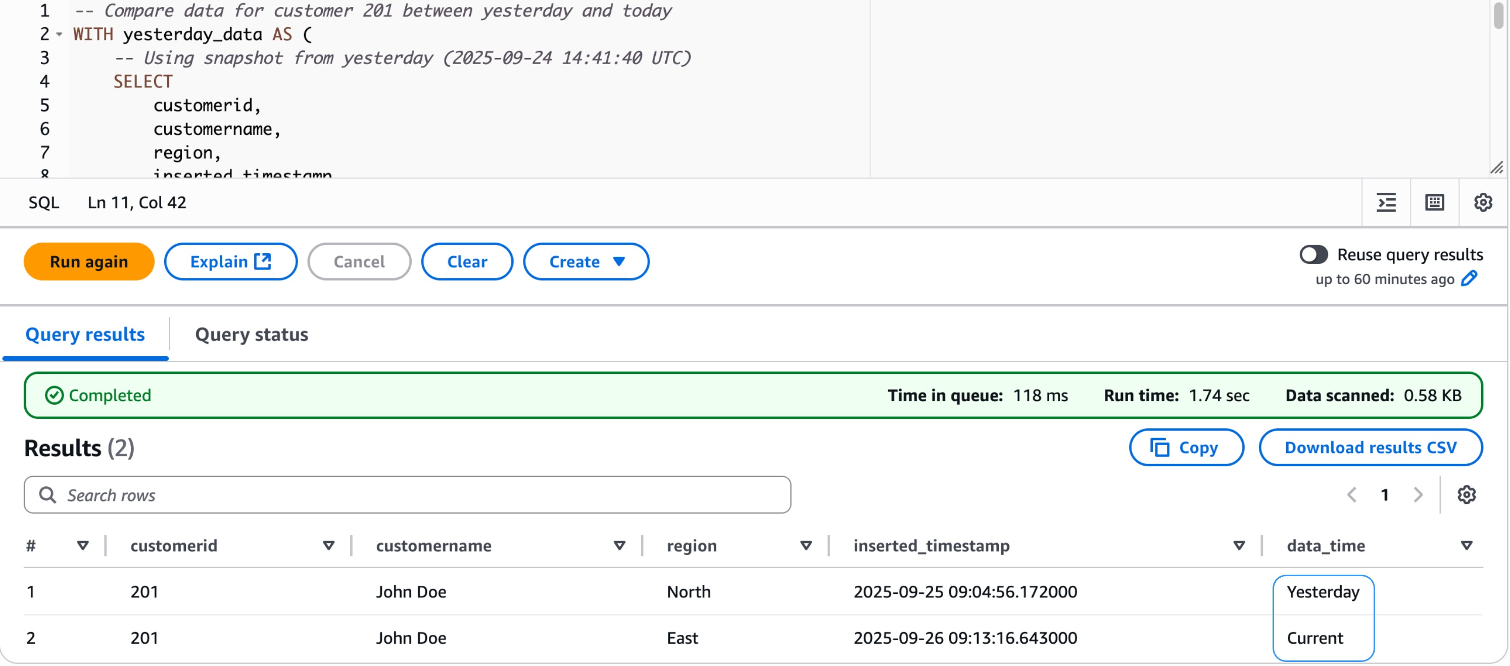
   Now, find the data state before and after the modification.

   

Step 7: Data quality tests

Data quality is a critical pillar of any reliable data pipeline. In this step, we define and enforce quality checks directly within the dbt project using schema-level test configurations. Rather than relying on one-time validation scripts, with dbt’s built-in testing framework, we can declaratively specify expectations on our models, ensuring that key fields remain unique, non-null, and consistent across the data layer before they reach downstream consumers.

1. Generic tests configuration

   The schema.yml file serves as the central contract for model integrity. Here, we apply generic tests on the fact_sales and dim_customers models to catch data anomalies early in the pipeline.

   # models/schema.yml
   version: 2
   
   models:
     - name: fact_sales
       columns:
         - name: orderid
           tests:
             - unique
             - not_null
         - name: salesamount
           tests:
             - not_null
   
     - name: dim_customers
       columns:
         - name: customerid
           tests:
             - unique
             - not_null

Step 8: Maintenance procedures

A well-functioning data pipeline requires ongoing maintenance to remain performant and auditable over time. This step covers two essential practices, table optimization to keep data storage efficient, and snapshot management to track historical changes in source data. Together, these procedures keep the pipeline reliable, cost-effective, and capable of supporting time-based analysis.

1. Table optimization

   As data accumulates in Delta or Iceberg tables, small files and fragmented storage can degrade query performance. The optimize_table macro provides a reusable utility to run Databricks’ OPTIMIZE command on any target table, consolidating small files and improving read efficiency without manual intervention.

   -- macros/optimize_table.sql
   {% macro optimize_table(table_name) %}
       {% set query %}
           OPTIMIZE {{ table_name }}
       {% endset %}
       {% do run_query(query) %}
   {% endmacro %}

2. Snapshot management

   To maintain a historical record of customer data changes, we use dbt snapshots with a timestamp-based strategy. The customers_snapshot model captures row-level changes from the raw source layer and persists them in a dedicated snapshots schema, enabling point-in-time analysis and audit trails.

   -- snapshots/customer_snapshot.sql
   {% snapshot customers_snapshot %}
   {{
       config(
         target_schema='snapshots',
         unique_key='CustomerID',
         strategy='timestamp',
         updated_at='inserted_timestamp'
       )
   }}
   
   SELECT * FROM {{ source('raw_sales_analytics_data_layer', 'customers') }}
   
   {% endsnapshot %}

Step 9: Monitoring and logging

Observability is an essential aspect of any production-grade data pipeline. This step establishes logging and monitoring practices within the dbt project to track pipeline runs, capture errors, and support debugging. With structured logging enabled, teams gain visibility into model execution, test results, and runtime behavior, streamlining issue diagnosis and maintaining operational confidence.

1. dbt logging configuration

   The dbt_project.yml logging configuration directs dbt to write logs to a dedicated path and outputs them in JSON format. JSON-structured logs are particularly useful for integration with log aggregation tools and monitoring dashboards, enabling automated alerting and audit trail management.

   # dbt_project.yml
   logs:
     path: logs
     enable_json: true

Step 10. Deployment and running

With the pipeline fully built, tested, and maintained, the final step covers how to deploy and execute dbt models across different scenarios. Whether running a complete refresh, processing incremental updates, or validating data quality, these commands form the operational backbone of day-to-day pipeline management.

1. Full refresh

   A full refresh rebuilds all models from scratch, reprocessing the entire dataset. This is typically used after significant schema changes, backfills, or when incremental state needs to be reset.

   dbt run --full-refresh

2. Incremental update

   For routine pipeline runs, incremental updates process only new or changed data, significantly reducing compute time and cost. The following command targets specific models (dim_customers and fact_sales) allowing selective execution without triggering the full DAG.

   dbt run --select dim_customers fact_sales

3. Testing

   After models are run, data quality tests defined in the schema configuration are executed to validate integrity across all models. This validates that constraints such as uniqueness and non-null checks are met before data reaches downstream consumers.

   dbt test

Step 11. Cleanup

1. Infrastructure cleanup

   # Delete EMR cluster
   aws emr terminate-clusters --cluster-id <cluster-id>
   
   # Remove S3 buckets
   aws s3 rb s3://amzn-s3-demo-transactional-datalake-raw-bucket-[unique-identifier] --force
   aws s3 rb s3://amzn-s3-demo-transactional-datalake-curated-bucket-[unique-identifier] --force
   aws s3 rb s3://amzn-s3-demo-transactional-datalake-analytics-bucket-[unique-identifier] --force

2. Database cleanup

   DROP SCHEMA raw_sales_analytics_data_layer CASCADE;
   DROP SCHEMA curated_sales_analytics_data_layer CASCADE;

Conclusion

In this post, you learned how to build a transactional data lake on Amazon EMR using dbt and Apache Iceberg, from environment setup and modeling raw data, to quality enforcing, snapshot management, and incremental pipeline deployment. The architecture brings together the scalability of Amazon EMR, dbt’s transformation capabilities, and Iceberg’s ACID-compliant table format to deliver a reliable, maintainable, and cost-efficient data platform.

To get started, see the Amazon EMR documentation to deploy this architecture in your own environment. Whether you’re modernizing a legacy data platform or building a new analytics foundation, this stack gives you the flexibility to scale with confidence.

About the authors