AWS Database Blog
Announcing distributed KV caching for self-hosted LLMs with Amazon ElastiCache
Today, we are announcing the general availability of fully managed distributed KV caching with Amazon ElastiCache for Valkey, a new capability that cuts self-hosted large language model (LLM) inference costs by up to 40% and time to first token (TTFT) by up to 80%. Distributed KV caching adds a shared cache next to the GPU fleet to store the key-value (KV) state inference engines compute during prefill. You connect your existing inference engines, including vLLM, SGLang, and TensorRT-LLM, through the open-source LMCache connector with only a configuration change and no changes to your code. In this post, we cover why prefill recompute is a bottleneck in self-hosted inference and how a distributed tier changes the cost. We walk through the architecture of the new capability and share performance results across industry benchmarks.
The compute bottleneck in self-hosted inference
Every token an LLM generates depends on the key and value tensors (KV state) produced for earlier tokens in the conversation. The engine keeps these tensors in memory as the KV cache. Think of it as notes on the chapters of a book that the model has already read: with the notes, the model does not need to read those chapters again.
An inference engine serves a request in two phases. During prefill the model reads the prompt and computes KV state for every input token in parallel. Prefill is compute-bound and grows quadratically with prompt length, because each token attends to all preceding tokens. Decode then generates output tokens one at a time. Each decode step reads the growing KV cache, so decode is memory-bandwidth-bound.
TTFT primarily reflects prefill latency and rises sharply with prompt length. Models take seconds to prefill a 32K-token prompt, tens of seconds for a 100K-token prompt, and minutes for contexts exceeding 250K tokens, in tests with B300 GPUs. AI coding assistants, support agents, and document question-answering pipelines push prompts past 100K tokens and repeat most of them across turns. Without cached KV states, the engine recomputes the entire prefill to process a short new message, including the system prompt, tool definitions, and every prior message in the conversation. Coding-agent traces, such as those from SemiAnalysis and TraceLab, show that over 95% of prompt tokens are part of previously processed prefixes. This repeated prefill can dominate GPU time, consuming capacity that could otherwise serve new requests.
How distributed KV caching helps
KV caching helps avoid prefill recomputation. A cached prefix skips the quadratic compute, and the engine prefills only the new tokens. Inference engines commonly cache KV state in two places. The first is GPU memory, the L0 cache. On today’s GPUs, that is up to 288 GB of HBM3e, shared between model weights and every request in flight. L0 is the fastest tier, but it is also the smallest, and the engine evicts older blocks to make room for new ones. Long conversations age out quickly. The second is host memory and local NVMe, reached through an offload library such as LMCache. This is the L1 cache. L1 is larger than L0 and close enough to the GPU to be useful, but it is private to a single server, and it competes with the rest of the server for memory. A request that lands on a different server misses it entirely.
These local tiers work well for short sessions that stay on one server. They break down for three common patterns:
- Long-running or returning sessions. A user returning after hours or days has fallen out of both L0 and L1 because those tiers are small and keep data for a short time. This is seen in coding agents, customer support assistants, and legal AI assistants where a prompt cache is limited to a few minutes.
- Routing shifts across the fleet. A request that lands on a different GPU server than the one that processed the prompt earlier misses reuse from local tiers. Traffic spikes force customers to choose between longer queues on GPUs with cached state and expensive recomputation on other GPUs.
- Server failures. Host failures and scale-in events could wipe local caches entirely. The fleet remains available, but latency rises as prompts need recomputation.
A distributed KV cache complements your existing L0 and L1 KV caches as a shared L2 tier for all GPUs in the fleet to share computed work. With an L2 cache, your KV cache survives GPU server boundaries. Returning users and spillover traffic can read KV state from the shared tier instead of recomputing it. The architecture can move from routing prompts to the server with KV state to fully using your GPUs, which helps reduce both the cost per million tokens and the TTFT.
For each request, the inference engine checks its local cache tiers in order and reads from the L2 tier only on a miss:
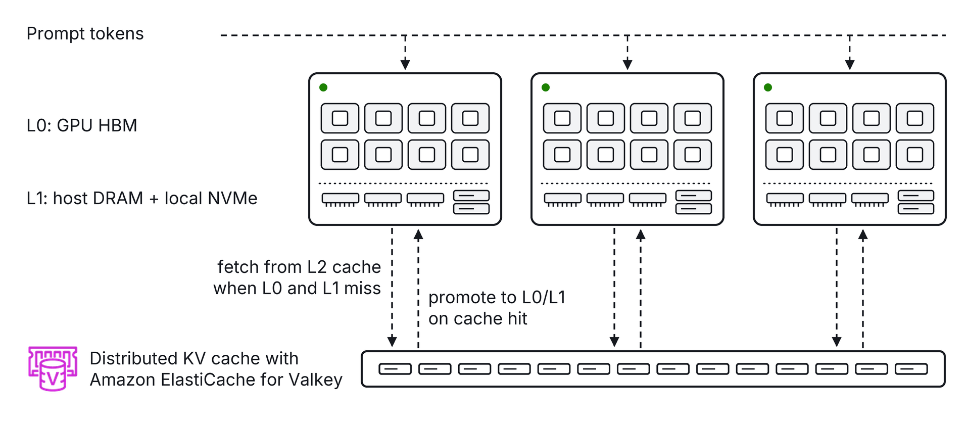
Figure 1: KV cache lookup across L0, L1, and the L2 distributed tier
When a request writes new KV state, the inference engine’s connector writes it to the L2 tier so any GPU in the fleet can reuse it on a future miss. vLLM, SGLang, and TensorRT-LLM can connect to the L2 tier through the open-source LMCache connector.
Distributed KV caching with ElastiCache
Distributed KV caching is a new capability that reduces self-hosted large language model (LLM) inference costs by up to 40% and TTFT by up to 80% using ElastiCache for Valkey. Distributed KV caching runs on cache.i8ge.48xlarge nodes in the same Availability Zone (AZ) as the GPU fleet and connects to GPUs through Remote Direct Memory Access (RDMA) over Elastic Fabric Adapter (EFA). This feature uses the newly introduced Valkey large-object support to store KV blocks in DRAM and NVMe.
Data tiering: ElastiCache for Valkey can read/write the hottest KV blocks from DRAM and tier colder blocks to the node’s local NVMe automatically. DRAM absorbs the active working set at line rate, and NVMe retains KV state cost-effectively for days, until the cache evicts it to make room. You interact only with the ElastiCache for Valkey endpoint.
RDMA over EFA: ElastiCache for Valkey can read and write large objects at millisecond latency using Remote Direct Memory Access (RDMA) with AWS Elastic Fabric Adapter (EFA) to transfer data between the GPU nodes and the cache nodes. RDMA moves KV tensors directly between the ElastiCache node’s memory and the GPU host’s memory, bypassing the operating system’s network stack, TCP/IP, and intermediate copies. This allows throughput of up to 220 Gbps per node. The cache itself responds in the sub-millisecond range for DRAM-resident blocks.
Distributed KV caching with ElastiCache provides petabytes of scalable storage, and every GPU in the AZ can read from the same L2 cache. A request can land on any server and still read its prior context from the L2 tier. When a GPU host fails, the surviving servers continue serving traffic and can read the KV state that the failed host wrote, as long as the cache has not evicted it. When traffic spikes force a new server into rotation, that server can read cached KV state from the L2 tier instead of starting cold.
Performance benchmarks and tuning your workload
Distributed KV caching with ElastiCache returns a multi-megabyte cache object from memory in under a millisecond, allowing retrieval of multi-GB KV states in milliseconds. Table 1 captures the latency that you can expect to retrieve and store 1 GB of data with cache.i8ge.48xlarge nodes, which support up to 220 Gbps at the time of publishing (November 18, 2026).
Table 1: Cache response time for large KV objects
| Object count | Cache action | Latency (P50) | Latency (P99) |
| One 8 MB object | Get | 477 µs | 950 µs |
| Set | 881 µs | 1,010 µs | |
| 1 GB (8 MB objects x 128, with one node) | Get | 41.7 ms | 42.1 ms |
| Set | 44.6 ms | 49.4 ms |
The cost and TTFT reduction benefits depend on your workload characteristics and the cache hit rate. We tested the performance of distributed KV caching with ElastiCache across different workload types and models, as directional guidance. We tested three common workload types, which include coding agents (SemiAnalysis Claude Code traces), AI assistants (Harvard FreeInference agentic trace, without Claude Code or SWE-bench), and long-context Q&A (LooGLE and L-Eval). We tested five different LLMs from 2026 with sparse and hybrid attention ranging from 250B to 1.6T parameters.
We tested the benefits for inference workloads using 2–6 P6 servers with 8 GPUs each, running vLLM. All baselines used GPU-local KV caching with about 150 GB of L0 and 205 GB of L1. The comparison runs added one cache.i8ge.48xlarge node in the same AZ using the LMCache Valkey connector.
Measured benefits for performance and cost
When GPUs fetch tokens from the cache instead of redoing prefill, they serve more prompts and cut TTFT. On the shared-document Q&A workload, each server handled twice the requests per second (RPS) with ElastiCache while maintaining interactivity. We define the interactivity service level objective (SLO) as TTFT under 5 seconds at p90 and time per output token under 50 milliseconds at p90. The doubling in RPS cut the cost per million output tokens by 40%, after paying for the ElastiCache node. At the same load, adding a shared cache across the GPUs provided lower TTFT and time per output token (TPOT), so answers start sooner and stream more smoothly.
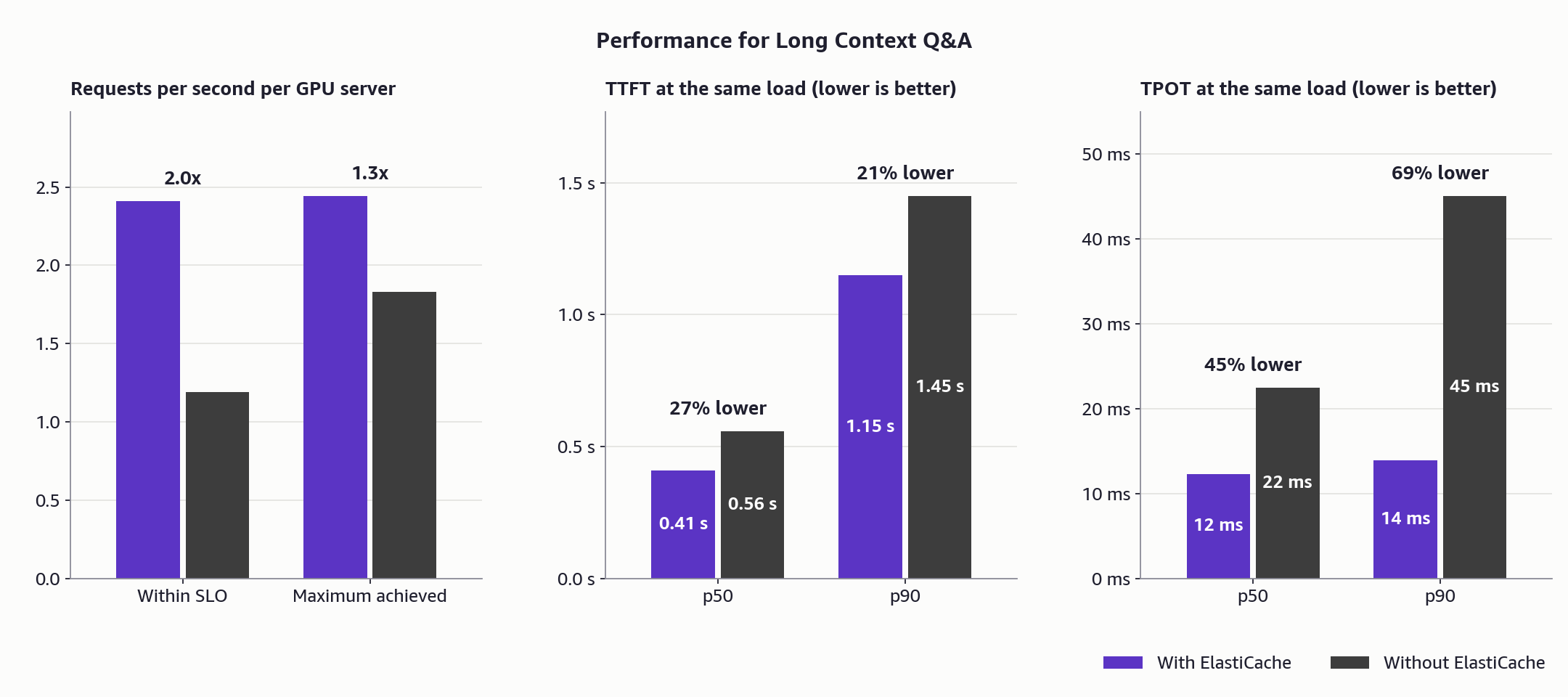
Figure 2: Performance for long-context Q&A workloads
We also tested coding agents and AI assistants with the SemiAnalysis AgentX methodology.
Across both workload types, each GPU server reached a 23% higher peak in tokens per second (token throughput) with ElastiCache. At the same load, ElastiCache delivered up to 1.98x the throughput for coding agents and 1.61x for AI assistants while staying within a p90 TTFT SLO of 30 seconds. We attribute the larger coding gain to the longer prompts typical of coding workloads.
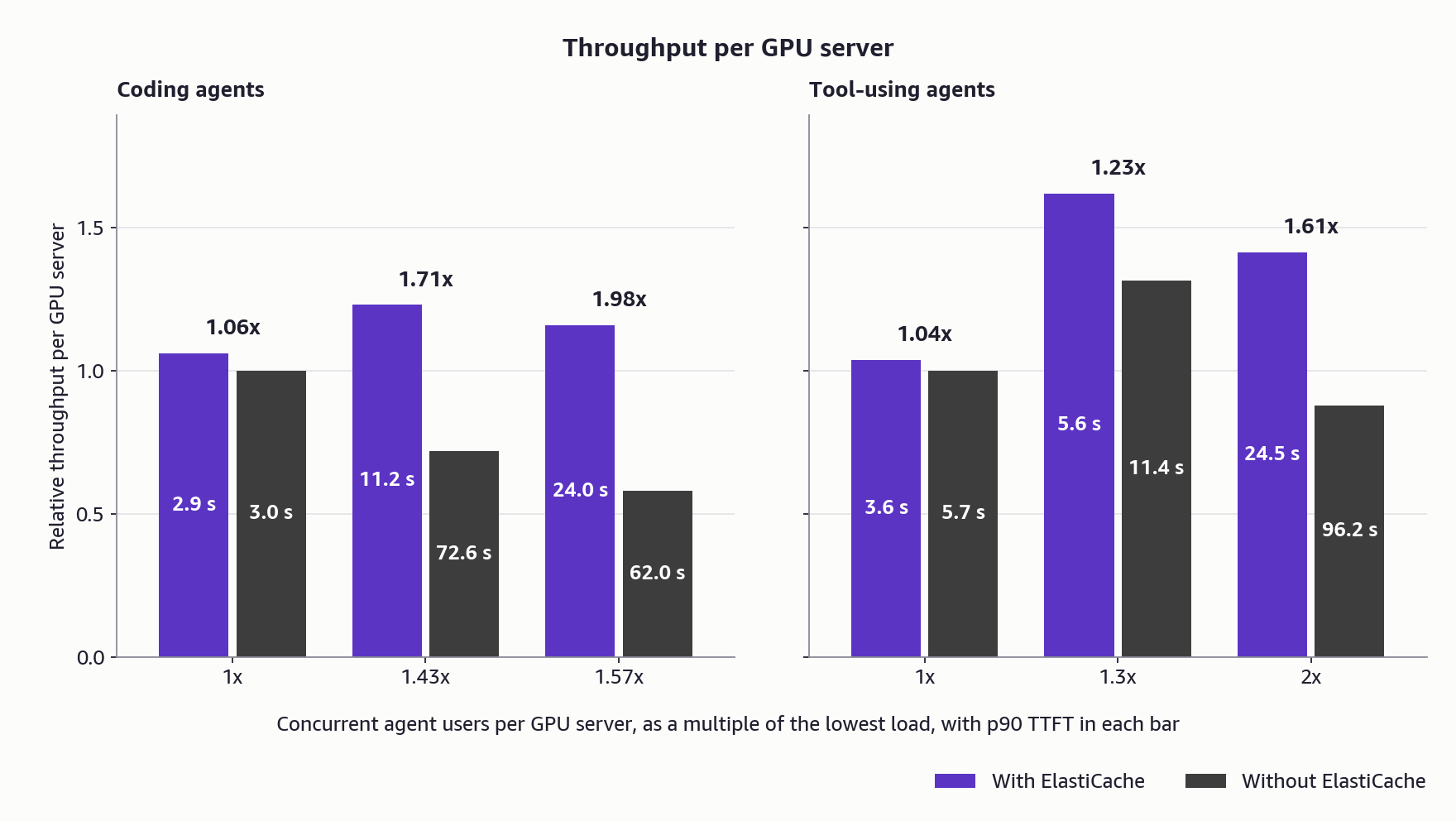
Figure 3: Performance for coding agents and AI assistant workloads
With a shared cache, the system performs better under GPU server failure, and hydrating the restarted server from the cache brings the system back to initial capacity faster. We tested a two-server system by stopping a server and then bringing it back up. With ElastiCache, the remaining server held p90 TTFT to 34.7 seconds over the first 300 seconds, 43% lower than without ElastiCache, while completing 1.48x the requests. Adding the server back returned the system to its initial throughput and TTFT within 60 seconds. Without ElastiCache, the system took up to 600 seconds to return to its original throughput, and queued requests still held p90 TTFT at 12.1 seconds.
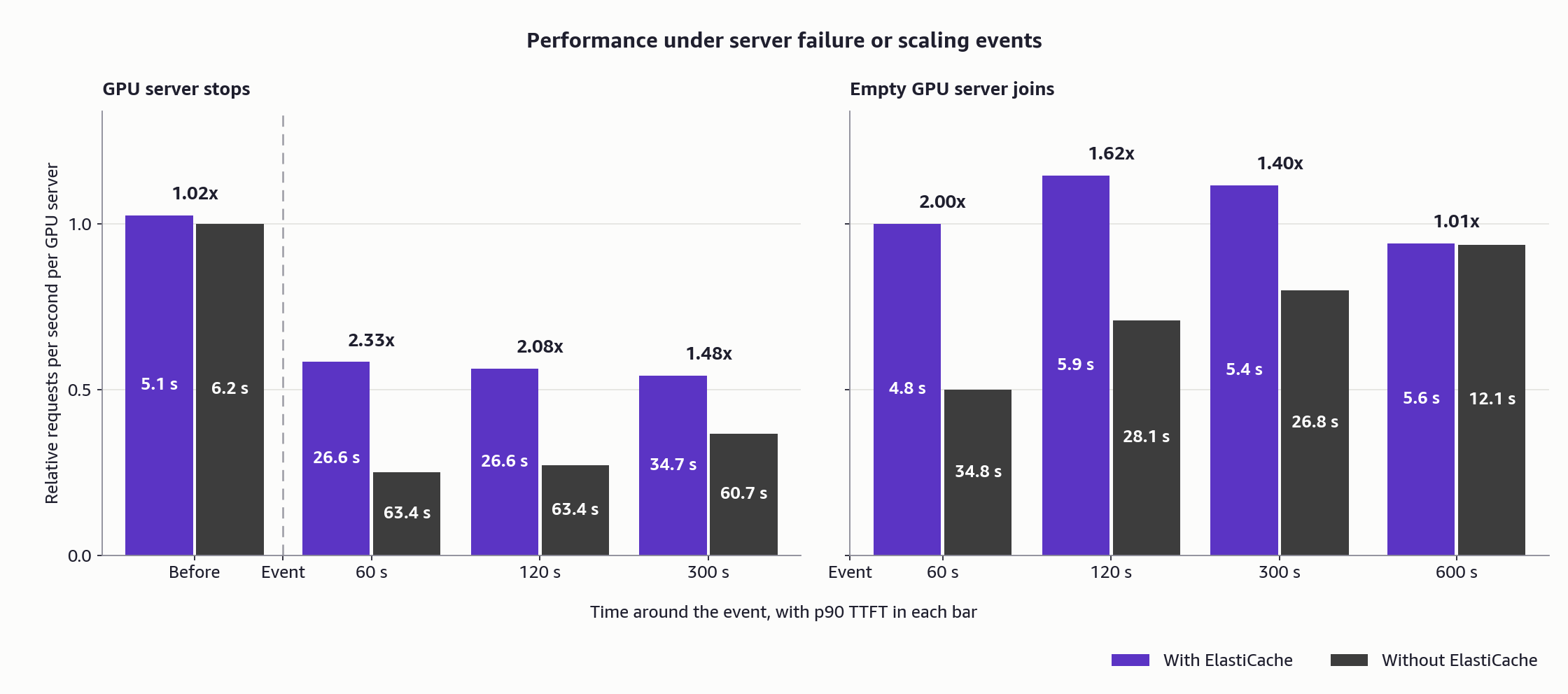
Figure 4: Server failure or scaling scenarios
A cache hit reduces the prefill work GPUs perform, which cuts TTFT. We saw TTFT reductions ranging from 55% to 93% from testing eight models across two full-attention, three sparse-attention, and three hybrid architectures. Full-attention models can see TTFT fall by 80% or more at prompts as short as 10K tokens. Similarly, sparse and partial-layer attention models see large TTFT reductions, because they store less KV per token, so a cache loads quickly while prefill recompute stays relatively expensive. Hybrid architectures provide smaller TTFT reductions at short lengths, but the reduction per cache hit grows to 84% past 100K tokens and up to 93% near 1M tokens. This is because hybrid attention models keep fixed-size states to reduce per-token KV cache size. At short context lengths, those states make up most of what a cache load fetches, so each load is comparatively large.
Each model has a cutover point, which represents the prompt length above which fetching from the cache is faster than recomputing. Every model in our test cuts over below 10K tokens, from under 512 tokens for a sparse model to between 1,000 and 7,600 tokens for hybrid models. If you are looking to primarily improve latency, we suggest finding the cutover point for your workload configuration and caching only prompts above it.
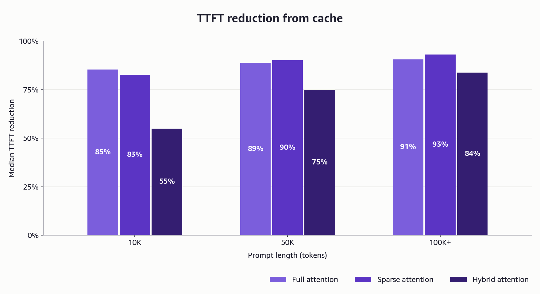
Figure 5: TTFT reduction per cache hit from reading a prompt prefix from ElastiCache, compared to a full recompute
Multiverse Computing ran distributed KV caching with ElastiCache for Valkey and shared their results.
“At Multiverse Computing, we help customers scale inference workloads with compressed models that cut costs and latency. We cut both even further and served more prompts on existing GPUs by adding distributed KV caching on ElastiCache for Valkey. With ElastiCache, we processed 50% more requests on the same GPUs within our one-second target for median time to first token. We achieved a 23% reduction in our median time to first token at normal traffic, and a 95% reduction at peak traffic.”
— Ennio Pastore, Director of AI Platform at Multiverse Computing
Workloads that benefit most
Distributed KV caching delivers the largest gains on workloads that match one of these patterns:
- Long input prompts with returning or shared sessions. AI coding assistants that work in the same codebase across many turns. Support agents that keep hours-long or days-long conversation histories. Document question-answering where many users ask questions over the same contracts or manuals.
- Traffic that spreads across many GPU servers with spiky arrivals or routing shifts. Inference providers that serve open-weight models across customers. Retail or ads workloads where a shared system prompt is combined with a user-specific tail.
Distributed KV caching provides less lift for small-scale deployments where KV state fits comfortably in GPU memory, for workloads that make a single LLM call with no reuse (classification, translation, moderation), and for applications that generate long outputs from short prompts.
Savings for your workload
You can use the open-source KVTrace tool to estimate the cost savings and TTFT improvements to expect for your workload before deploying distributed KV caching, at no additional charge. KVTrace uses the cache events that vLLM and SGLang already publish for your inference workload and reports the missed recompute that a distributed KV cache would have served. KVTrace provides close estimates of expected cache hit rate, cost reduction, and TTFT reduction for your traffic mix along with the recommended cluster size to capture these benefits. KVTrace uses the arrival times and the size of KVs for your application’s traffic, then simulates the benefits at different L2 cache sizes offline. KVTrace is safe to run estimates on your production cluster because it does not require changes to your inference engine or GPU clusters. It preserves prompt data privacy by using only hashed prompt data. Follow these steps to use KVTrace with vLLM.
Conclusion
Distributed KV caching on Amazon ElastiCache for Valkey cuts cost per million tokens by up to 40% and TTFT by up to 80% for self-hosted LLM inference. You can run the KVTrace tool to size the benefits for your inference traffic before deploying any infrastructure, without any charge. You can get started by using the AWS Command Line Interface (AWS CLI) within your terminal by creating an ElastiCache for Valkey cluster in the same AZ as your GPU fleet and adding the endpoint to your inference engine. To learn more, visit the ElastiCache documentation.